Explore the tools and data
A bluespot is simply another term for a landscape depression originally defined by the Danish Road Directorate in a report aimed at presenting the storm water consequences on infrastructure. It puts a special emphasis on flood risk: A bluespot is an area likely to fill or overflow in a storm water situation, endangering structures located within or near it.
On the evening of July 2, 2011, downtown Copenhagen, Denmark, was hit with 136 millimeters of rain (nearly 5 inches) in an hour and a half. The overwhelmed sewer system backed up, causing thousands of basements to be flooded with a mixture of rain and wastewater. In the aftermath of the storm, insurance companies paid about $1 billion in compensation to some 90,000 policyholders.
The aim of this series of lessons (organized as modules) is to predict flood risk assessment due to storm water incidents and to consider where to avoid future site developments while considering the effect of future climate changes. These lessons replace and build on an older set of tools and lesson and incorporate hierarchical downstream spillover.
Model predictions explored in these lessons are based on the screening of a digital terrain model for landscape depressions within a drainage basin, their hierarchical downstream locations, and how they fill up and spill over during simulated uniform rainstorms while ignoring local infiltration rates and time. Where building footprints are available, these may be incorporated into the digital terrain model from the beginning, thereby allowing the model to predict impacts on infrastructure and other land uses.
For an introduction to bluespot modeling, review Coping with Cloudbursts.
Bluespot modeling - setup
In this lesson, you will explore a drainage basin north of Copenhagen, Denmark, that has been severely impacted. Many residential homes and other critical infrastructure are located within landscape sinks that are filled during a rainstorm, thus flooding homes and affecting roads and rail tunnels. Using the tools (models and scripts) and the sample dataset provided, you will model and predict flood consequences for a series of simulated storm water events.
The lesson objectives include the following:
- Introducing the overall flood risk screening method, workflow, and tools
- Introducing storm water incidents and the impacts on society in times of climate changes
- Installing and setting up the modeling project
- Investigating input data requirements and sample data for the Charlottenlund area north of Copenhagen, Denmark
- DTM
- Building footprints
- Roads
- Railroads
Note:
These lesson modules require ArcGIS Pro 2.6 or later with an ArcGIS Spatial Analyst extension license. A third-party Python plug-in named networkx is not included and configured in older versions of ArcGIS Pro and thus may require additional installation and configuration.
- Download the Bluespot Screening zip file to a folder of your choice.
Consider creating and using C:\Charlottenlund_Stormwater as a folder location.
- Unzip the file and use Windows File Explorer and verify the contents of the folder.
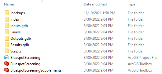
- In the folder, locate and double-click BluespotScreening.aprx to launch ArcGIS Pro. If prompted, sign in using your licensed ArcGIS account.
Note:
If you don't have access to ArcGIS Pro or an ArcGIS account, see options for software access.
The BluespotScreening project opens and displays a map with the imagery basemap and several modeling data layers. You may notice a datum transformation warning, you can ignore this. Before getting started, you may need to verify whether the Spatial Analyst extension is available.
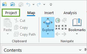
- On the ribbon, click the Project tab.
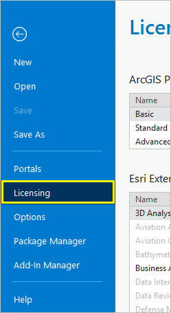
- In the list of tabs on the side pane, click Licensing.
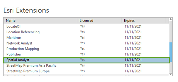
- In the Licensing pane, locate Esri Extensions and verify that Spatial Analyst is licensed.
Before proceeding, you will review the current installed Python packages to determine whether the necessary networkx package is available, installed, and configured.
- On the side pane, click Package Manager.
- In the Package Manager pane, for Active Environment, verify that the current project environment is set to the arcgispro-py3.

Note:
You may have a different project environment selected. ArcGIS Pro supports multiple configurations and allows you to switch and manage environments used for different applications. If your project environment is not set to arcgispro-py3, use Environment Manage to switch.
- If necessary, in Package Manager, click the Installed tab.
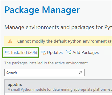
- In the Installed Packages list, search and locate the networkx package.
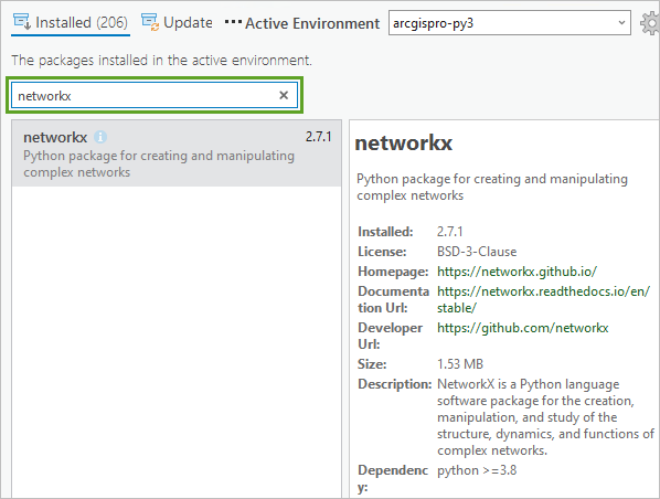
Note:
Newer versions of ArcGIS Pro include installation of the networkx package. If you are unable to verify the networkx package is installed, you may want to upgrade to a more current version of ArcGIS Pro.
- On the side pane, click the back arrow to return to the project.
Next, you will verify that the NetworkX Python plug-in is accessible in ArcGIS Pro.
- On the ribbon, on the Analysis tab, in the Geoprocessing group, click the Python drop-down arrow and choose Python Notebook.
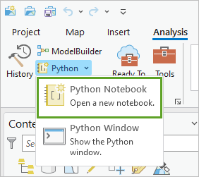
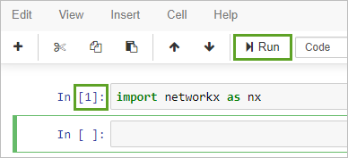
- In the New Notebook (1) window, type the following line of code:
import networkx as nx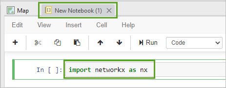
- Click Run.
While the cell runs, an asterisk is inside the brackets in the input area so it appears as In [*]. After the cell finishes running, the number 1 replaces the asterisk in the brackets. When the notebook returns 1, it indicates that the package is configured and you may continue.
- Close the New Notebook window.
- On the quick access toolbar at the top, click Save to save the project.
Next, you will explore the sample data and modeling tools needed to run the bluespot model.
Bluespot modeling - model tools and data
In this section, you will review the sample data for Charlottenlund, as used in the BlueSpotModel project and used in this storm water assessment.
- In the Catalog pane, expand Folders, then expand Charlottenlund_Stormwater (or the folder used to unzip the project files).
All project data is stored in file geodatabases, and input data is separated from output data in different geodatabases. In addition, the project has several subfolders containing project layer files, scripts, and the model tools.
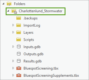
Note the following:
- The Charlottenlund_Stormwater folder is the project folder (yours may differ).
- The Scripts folder is a location to store project scripts.
- The Inputs.gdb geodatabase contains input sample data.
- The Outputs.gdb geodatabase contains user-generated output data.
- The Results.gdb geodatabase contains results as generated by the modeling.
- The BluespotScreening.tbx file is a toolbox with models and script tools.
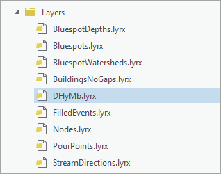
- Expand and review the Layers folder.
The folder contains layer files with symbology ready to import.
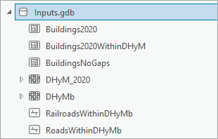
- Expand and review the Inputs.gdb geodatabase.
The Inputs geodatabase contains the necessary input data to carry out the storm water screening and bluespot modeling.
Bluespot modeling – data requirements and workflow
Using the project data and tools, you will discover where excess water flows downstream, shaping an often highly complex network of streams contributing to the fill-up of other bluespots until the spillover finally reaches the ocean.
Typical bluespot modeling data requirements are as follows:
- Your data must be in a projected coordinate system and both the horizontal and vertical units must be metric, as all area and volume calculations used by the bluespot modeling tools require this.
- A raster-based digital terrain model (DTM) representing levels on ground obtained by high-resolution lidar technology is preferred, but lower-resolution terrain models may provide useful results, too.
- If possible, the DTM should be hydrologically conditioned, in other words, corrected for water passing under infrastructure. A digital surface model (DSM) will not provide trustworthy screening results, as it represents a combination of levels on bare earth, on top of buildings and vegetation.
- The inclusion of vegetated surfaces will cause significant errors in the modeling of flow paths, locations of landscape depressions, their volumes, pour points, and associated watersheds.
- Ensure that no filtering methods were used in a post-processing step during the removal of vegetation and building features from the DSM to obtain the ground levels for a DTM. If that were the case, landscape depressions would not have true depths.
- However, as the method used is based on flow calculations on ground, the inclusion of buildings is fine to divert water around them. An optional polygon feature class of building footprints is beneficial and can be used to elevate buildings and stamp (imprint) them onto a DTM, as this will allow water to be diverted around buildings (unless raised on pillars). Furthermore, the volume occupied by buildings when located in depressions should be subtracted when assuming that water cannot flow into their basements.
Note:
- If data is unprojected and horizontal and vertical units are not metric, project the data.
- If the DTM is not clipped to a drainage basin, derive basins and clip the DTM to match a basin.
- If building footprints are available, dissolve buildings and imprint them into the DTM.

In the Run the model and tools lesson module, you will investigate the sample data in more detail and step through the storm water screening’s process, followed by a quick inspection of the results. These steps are as follows:
- Step 1: Identify Bluespot Features
- Step 2: Create Nodes and Edges
- Step 3: Prepare Fields
- Step 4: Spillover Batch
- Step 5: Filled Events
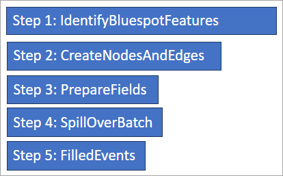
In the Explore the results lesson module, you will assess the modeling results and assemble the full picture from the results and discuss the storm water consequences at different scenarios.
Finally, in the Run the analysis with your own data lesson module, you will explore the data requirements and steps needed to use the bluespot modeling tools with your own data.
When you are ready, move to the next module and start following the steps to explore the sample data and use the tools (models and scripts) to predict flooding consequences for a series of simulated storm water events.
Run the model and tools
In this module, you will review and explore the Charlottenlund sample dataset and use the tools (models and scripts) to predict flooding consequences for a series of simulated storm water events. The study location is a drainage basin north of Copenhagen, Denmark, where impacts are severe, as many residential areas are located in landscape depressions that are filled up partly or in full during a rainstorm, thus flooding many homes and also affecting other critical infrastructure. You will step through the storm water screening's process followed by a quick inspection of the results
In the next module, you will assess the modeling outputs and gain a better understanding of storm water consequences at different storm scenarios. The goal is to predict the overall consequences of storm water to various societies and consider where to avoid future site developments without taking the necessary precautions in times of climate changes.
The predictions are based on the screening of a digital terrain model for landscape depressions within a drainage basin, their hierarchical downstream locations, and how they will be filled up and spill over during simulated uniform rainstorms neglecting local infiltration rates and time.
The lesson goals include the following:
- Inspecting the sample data provided
- Running the models and scripts
Inspect the sample data
You will start by exploring the basic dataset involved in bluespot modeling: layers include a DHyMb raster, which is a hydro-conditioned digital terrain model (DHyM) and a layer of building footprints. Furthermore, you will explore at the building layer, used to create the modified DHyMb, and two layers showing the occurrences of roads and railroads that may be used later when interpreting your results.
- If necessary, open the BluespotScreening project.
The project has several bookmarks to assist in locating various landmarks and areas of interest identified in the model results.
- On the Map tab, in the Navigate group, click the Bookmarks drop-down menu.
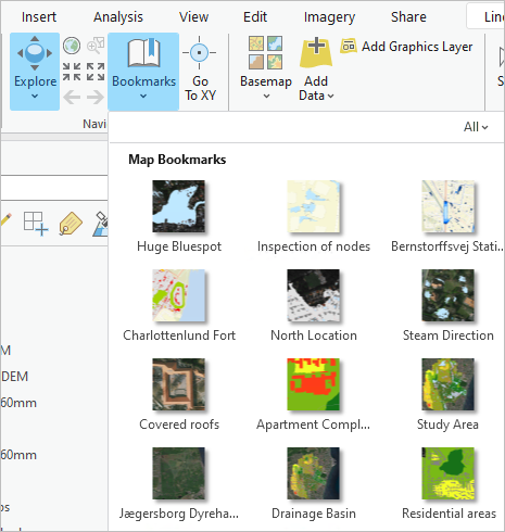
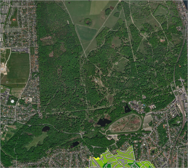
- Click the Study Area bookmark to ensure the map displays the extent of the study area.
- Use the Explore tool to pan and zoom and investigate the drainage basin that serves as the study area for this lesson.
Notice that the catchment it is located in the North of Copenhagen, Denmark.
- Use the Jægersborg Dyrehave park bookmark to explore this popular recreation site used by citizens. The park’s history can be dated to 1669 during King Frederik III reign, when it was used for deer hunting.
- In the Catalog pane, expand Folders and BluespotScreening.
- Expand the Inputs.gdb geodatabase.
The feature classes in the Inputs geodatabase represent processed data used in the tools and models to predict the flooding consequences for a series of simulated storm water events.
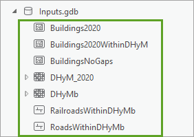
The data is already added to the map as a collection of layers organized in the Contents pane. The layers are organized with line layers displayed above polygon layers and raster layers located below polygon layers.
Next, you will use the Explore tool to pan and zoom and investigate the drainage basin.
- Use the Drainage Basin bookmark to zoom to the extent of the Charlottenlund storm water basin.
- In the Contents pane, if necessary, check the check box next to each of the following layers: BuidingsNoGaps, RailroadsWithinDEM, RoadsWithinDEM and DHyMb layers.
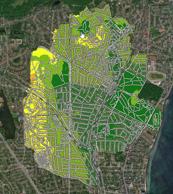
The RailroadsWithinDEM and RoadsWithinDEM layers show the locations of all minor and major roads and railroads located within the drainage basin. When comparing your screening results with these layers in the Explore the results lesson, you will be able to identify which parts of the infrastructure are most affected by floods.
- Use the Residential areas bookmark.
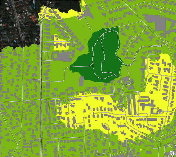
The map shows several residential areas containing a mixture of single-family homes and apartment blocks.
- On the Map tab, in the Navigate group, click Explore and investigate the BuildingsNoGaps layer and zoom in to several building roofs.
- Use the Covered roofs bookmark to zoom to the extent of a closed building complex.
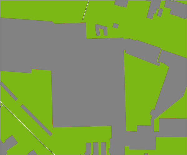
During the data preparation phase of the project, a roof was “added” to prevent precipitation from being trapped inside the courtyard. This preparation step will be demonstrated in the Run the analysis with your own data lesson.
- In the Contents pane, uncheck the BuildingsNoGaps and DHyMb layers to investigate a building with an open courtyard.
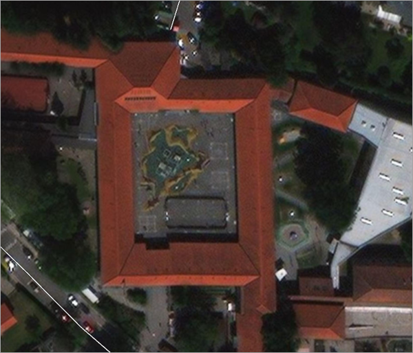
- Use the Apartment complexes bookmark to investigate an additional closed building complex.
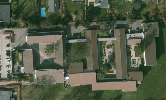
- In the Contents pane, check the BuildingsNoGaps layer to investigate how a roof was added to prevent precipitation from being trapped inside the courtyard.
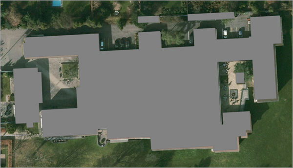
- Check the DHyMb layer.
- In the map, use the Explore tool to investigate the RoadsWithinDEM and RailroadsWithinDEM layers.
Notice that the railroad lines stand out clearly but are only passable through road overpasses or road underpasses built at several locations.
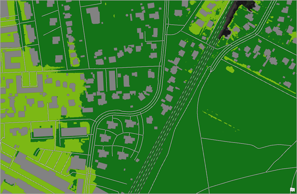
You will explore and investigate some of the critically impacted underpasses in the next lesson, in which you will also consider the flood impacts on residential areas.
- In the Contents pane, uncheck the BuidingsNoGaps, RailroadsWithinDEM and RoadsWithinDEM layers.
- If necessary, expand the DHyMb layer.
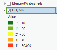
The DHyMb layer is a raster layer with cell values representing elevation above sea level in meters for the hydrologically adapted DTM covering the Charlottenlund drainage basin.
Note:
If possible, the DTM should be hydrologically conditioned, in other words, corrected for water passing under infrastructure. A digital surface model (DSM) will not provide trustworthy screening results, as it represents a combination of levels on bare earth, on top of buildings and vegetation. As the method used is based on flow calculations on ground, the inclusion of buildings is fine to divert water around them.
- In the map, use the Explore tool to pan and zoom and investigate the DHyMb layer. Notice that darker green represents low-lying areas prone to flooding and orange and red areas represent higher-lying areas less likely to flood.
While reviewing the terrain model’s sliced elevation values, you may start to get a first impression of where the water moves from the higher elevation boundary of the drainage basin toward the lower elevation dark green region in the central and eastern parts.
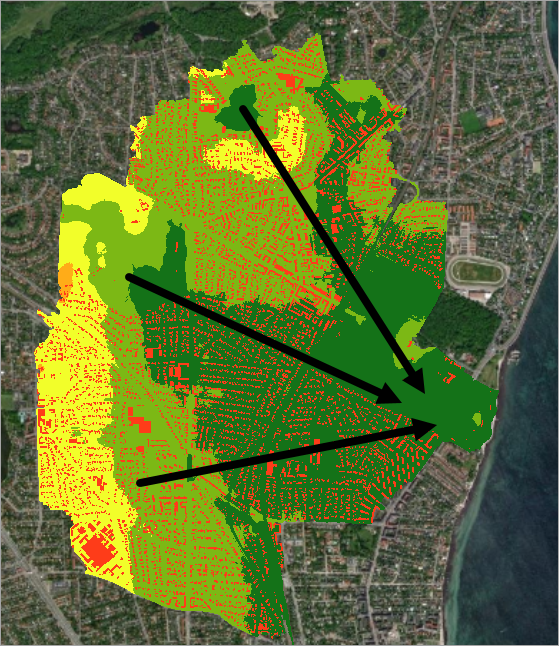
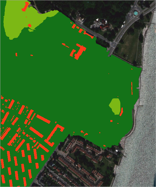
The basin has an outlet into the sea east of the Charlottenlund Fort, which was constructed from 1883–1888 with the goal of protecting the entrance into the Copenhagen Seaport.
- Use the Charlottenlund Fort bookmark to investigate the basin outlet.
- Use the Explore buildings bookmark and the Explore tool, then click some of the buildings in the DHyMb layer.
Notice that buildings are assigned a very high elevation value (30,000) to enforce storm water runoff around them.
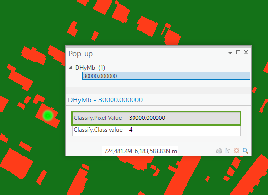
- Close the Pop-up when done.
- In the Contents pane, right-click Map, then choose Properties.
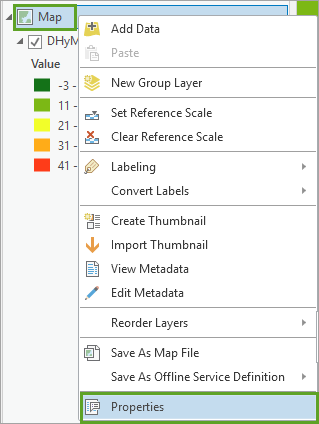
- In the Map Properties pane, click Coordinate Systems and review the current coordinate system settings.
Note:
Your data must be in a projected coordinate system and both the horizontal and vertical units must be metric, as all area and volume calculations used by the bluespot modeling tools require this. In this study, the map coordinate system is defined as ETRS 1989 UTM zone 32N with a SRID of 25832.
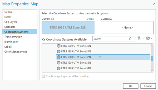
Notice that the horizontal spatial reference system for all data used in the map is ETRS 1989 UTM zone 32N, which is a UTM projection with the ETRS89 datum applied. This is the most commonly used spatial reference system for Danish maps with horizontal and vertical units for 3D features in meters.
- In the Map Properties pane, click Cancel.
- Click Save to save the project.
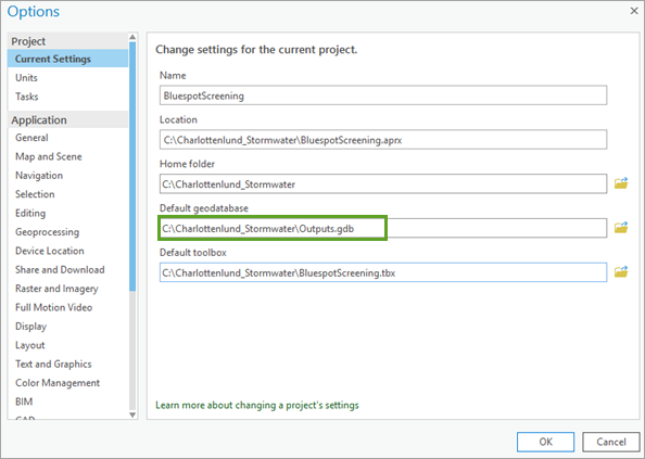
To ensure that the modeling tool outputs are saved in the correct output workspace, you must make sure that the projects default geodatabase is correctly set.
- Click the Project tab, then click Options.
- In the Options pane, review the current settings for the project.
- Verify the Default geodatabase is set to the Outputs.gdb geodatabase, which is located in your home folder (for example, C:\Charlottenlund_Stormwater\Outputs.gdb).
With the default geodatabase set, results from geoprocessing operations will automatically be directed to this location. Meanwhile, you will notice that some models and script tools include an Output Workspace parameter as well. This is to make sure that outputs from geoprocessing tools referenced as sub-components within other models or scripts are saved in the right location.
- When done, click OK.
- On the Project tab, click the Back button.
Review the model and tools
A bluespot is a landscape depression, big or small, where precipitation is trapped during heavy rainfalls. In this section, you will investigate the model and associated tools.
The following illustration shows a cross section of a local bluespot catchment with precipitation falling onto the terrain. The bluespot begins to fill (assuming Hortonian flow conditions) and when it reaches capacity, it spills over at its so-called pour point.
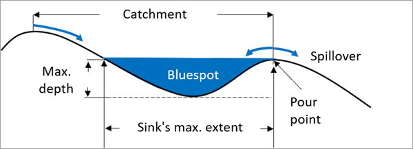
Located in the project's BlueSpotScreening toolbox is a model named Identify Bluespot Features. The purpose of the model is to detect the bluespots, their pour point locations, and the downstream flow paths when the bluespots spill over.
Initially, the model detects all bluespots—no matter their depth or volume. Meanwhile, to get the bigger picture of where storm water gets trapped and may cause problems to buildings and infrastructures, a filter is introduced, eliminating the smallest insignificant bluespots from the calculations. This filter is a combination of depth and volume criterions, so very shallow bluespots with small volumes may be left out intentionally to reduce the computations and limit the outputs. For example, when working on the current dataset, we want to eliminate depressions where the maximum depths are less than 5 cm, in accordance with the z-limit threshold shown in the illustration above and having volumes smaller than 1 m3. When using these threshold values, you will see in a short while that a total of 3388 bluespots are found, but without the threshold, the number would have been a stunning 680770 bluespots that would have been detected. Of course, this means that the total volume stored in the tiny bluespots is left out of the calculations as the ‘lost’ bluespot capacities are turned into surface runoff that might be subject to error analysis. However, in that context, bear in mind that in general, it is considered best practice not to search for bluespots shallower than the vertical accuracy for the elevation model used, which in this case is 5 cm.
Thus, puddles located along infrastructure (or on farmland in between plough furrows) are ignored, but deeper and more voluminous bluespots located elsewhere are preserved. Meanwhile, if you work for a road authority, you may want to keep bluespots in the analysis that are shallow but smaller than 1 m3 by volume (= 1,000 liters) to identify dangerous hydroplaning locations for cars—or if you want to identify holes along bike lanes or curbsides cut off from drains that could impair bikers and result in dangerous situations for others. When identified, such bluespots may be leveled out at the next road maintenance service.
DTMs are per definition representations of terrain levels on ground and could include buildings imprinted into the terrain. As precipitation (when modeled) should be diverted around buildings, it is important to leave out building volumes if located inside bluespots.
Next, you will explore and review the Identify Bluespot Features model.
- In the Catalog pane, expand Toolboxes and expand BluespotScreening toolbox. Locate the Identify Bluespot Features model.
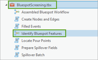
- Right-click the Identify Bluespot Features model and choose Edit.
- If necessary, reposition the model window and fit the model to the window.
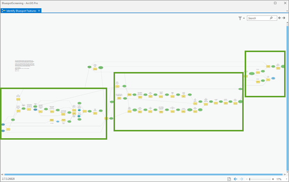
At first glance, the model may seem rather complex, but when exploring its various components, you will notice that parts of the model focus on specific aspects of the workflow.
- The left part focuses on determining the surface flow and identifying the bluespots using raster-based tools.
- The central part executes the LocatePourPoints tool, which is a Python script tool to identify the bluespot pour points.
- The right part is mostly about converting the identified bluespots and local watersheds into vector representations, assigning meaningful attribute names to the outputs and joining tables.
- In the Model window, pan and zoom in to the left part of the model and review the tools and parameters.
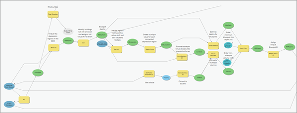
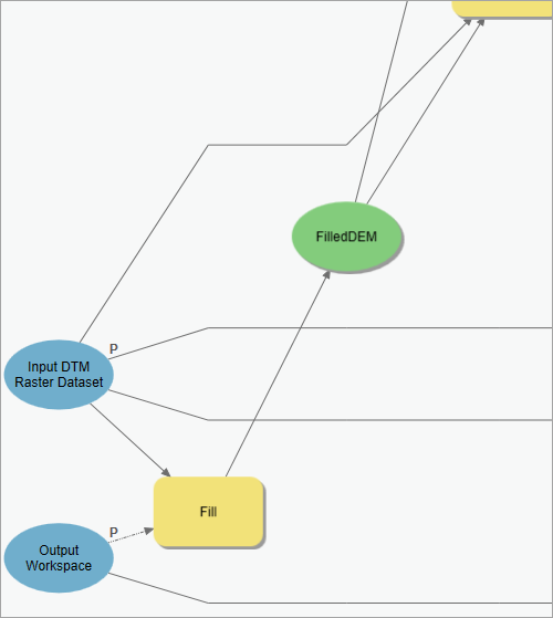
Note the sequence of Spatial Analyst tools used to identify the bluespots’ spatial extents by first filling up all landscape depressions detected in the DTM to their pour point levels.
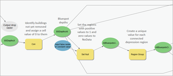
Next, the original elevation values in the Input DEM are subtracted cell by cell from DEMFilled to create a depth raster of all depressions named BSDepths. Afterward, the individual bluespots are assembled by using the Region Group tool.
In addition, notice how a bluespot's volume is calculated by multiplying all cell values in the BSDepths raster by the area of a cell (in the sample dataset, the cell size is .4 * .4 = .16 m2) and then summarizing all values. This is done by using Zonal Statistics and the Volume Calculator tools. The criteria used to ignore small sinks is handled by the Apply Filter tool.
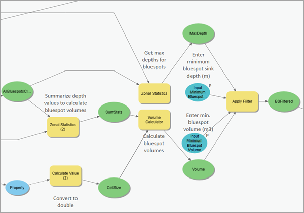
Next, a bluespots pour point is determined by the LocatePourPoints script tool from a search for the cell within a bluespot that has the highest flow accumulation value.
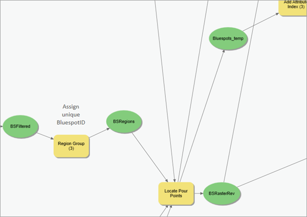
Meanwhile, since the pour point is located along a bluespot’s rim, it isn’t included in the its extent. Therefore, the pour point is moved to the next downstream cell that has a higher flow accumulation value just outside the bluespot using the SnapPourPoint tool. Next, the bluespot is expanded to include the pour point cell, also, before calculating the bluespot’s local watershed using the Watershed tool.
Note:
It is open for discussion, if the entire rim for the bluespot should be included as part of the bluespot, but as a bluespot’s depth for each cell along the rim is zero, it is not included here. However, from a technical point of view, a bluespot’s local watershed may be bigger when including the rim’s cells as the input to the Watershed tool.
How surface runoff is derived from a DTM and how to identify the bluespots pour points is discussed in the following help topics: How Flow Direction works and How Flow Accumulation works. These topics describe how the steepest flow is calculated from each elevation cell and into its eight surrounding neighbors.
Flow direction and flow accumulationWhen flow directions are identified, the flow accumulations describe how the downstream flow merges into minor streams and further downstream into larger river systems. In the illustration below, a DTM (a) is examined for steepest flow directions (b) on a cell-by-cell basis. Next, based on an encoding schema (c), the flow directions become more evident when visualized as arrows (d). The flow accumulation numbers in (e) tell how many upstream cells contribute runoff to a specific cell (e).
On your own, try to verify the flow accumulation number in (e) for the cell with the value 7 by walking upstream in (d).
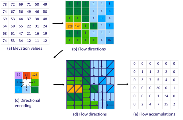
In the perfect DTM presented above (with elevation values rounded to integers) for a square drainage basin represented by 6x6 cells, all cells contribute to the lower cell with the value 35, and from that one all water leaves in a ‘downward’ direction. In this DTM, there are no local bluespots.
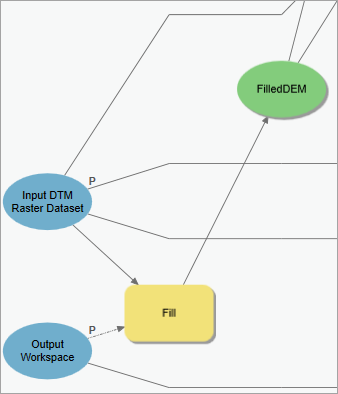
If bluespots were present, the flow directions would end in the lowest lying cell inside it. Therefore, to model a continuous flow for an entire catchment, we fill up all bluespots to their pour point levels using the Fill tool before calculating the flow direction. For a detailed discussion, review the help topic How Fill works.
In the Identify Bluespot features, all landscape depressions are filled based on the Fill tool, which leads to the identification of the desired bluespots.
Finally, the Streams feature class is derived from looking up the steepest downstream paths from all pour points determined by Spatial Analyst’s Optimal Path As Line tool found in the model’s upper right corner.
When using pour points as source cells, flow paths are determined from a "Look up" of the downstream flow directions from cell to cell in the FDFilled raster. The Flow Accumulation raster, FAFilled, is also a required input to this script tool.
Note:
Review the help topic Optimal Path As Line for more information about the tool.
The output from the tool is flow paths as line features with downstream directions. When lines from various pour points merge, overlapping lines are turned into single line features using the Create network paths option. As a result, the lines and points locations are ready for the next steps in creating the hydrologic network.
- When done reviewing the Identify Bluespot features model, close the model window and do not save any changes.
- Click Save to save the project.
Next, you will execute the model.
Run the Identify Bluespots Features model
To run the Identify Bluespots Features model, complete the following steps:
- In the Catalog pane, double-click the Identify Bluespot Features model.
The Identify Bluespot Features geoprocessing tool opens.
- In the Identify Bluespot Features geoprocessing tool, update the following parameters:
Note:
If your OS is set up to use a comma as a decimal separator, enter all decimal values with a comma.
- For Input DTM Raster Dataset, browse to DHyMb located in the Inputs.gdb geodatabase.
- For Input Minimum Bluespot Depth, type 0.05 (meters).
- For Input Minimum Bluespot Volume, type 1 (cubic meter).
- For Output Workspace, specify your Outputs file geodatabase.
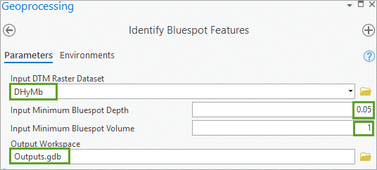
- Click on the Environments tab. Expand Parallel Processing and set the Parallel Processing Factor to 0.
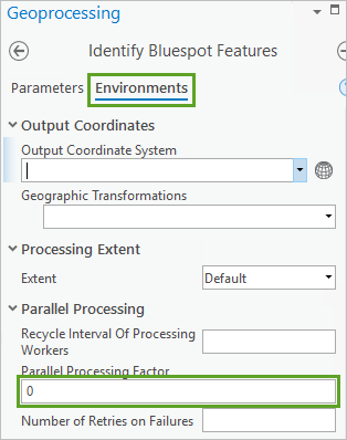
- Verify all parameter settings, then click Run.
Note:
Model execution time is between 10 and 15 minutes. You may monitor output messages from the model by choosing View Details in the geoprocessing tool.
Next, you will explore the model outputs.
- In the Catalog pane, expand Folders and Charlottenlund_Stormwater.
- Expand Outputs.gdb and review the model outputs.
Identify model outputs such as Bluespots, PourPoints, BluespotWatersheds, and BSDepths.
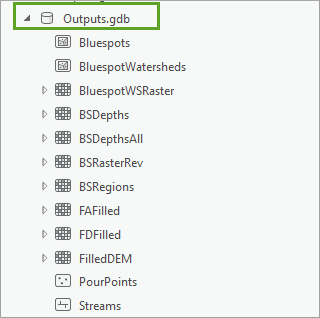
- In the map Contents pane, verify the following layers have been added and symbolized. If necessary, update and modify the symbology as described below.
Layer name Symbology PourPoints
6 pt. red dot
Bluespots
Light blue
BSDepths
Grayscale
Streams
Dark blue (arrows to be added later)
BluespotWatersheds
Light gray with visible outline
Note:
If a layer does not automatically update on the map, drag it from the Catalog pane, onto the lesson.
- In the Contents pane, if necessary, move and organize the layers as per the following:
- BuildingsNoGaps
- PourPoints
- Streams
- Bluespots
- BluespotWatersheds
- In the Contents pane, uncheck the DHyMb and the BSDepths layers.
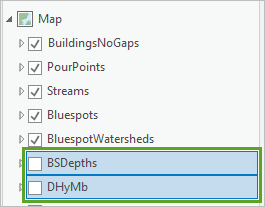
- Use the Huge Bluespot bookmark to explore the northernmost part of the study area. On the map, inspect the locations of buildings, bluespots, and their local watersheds.
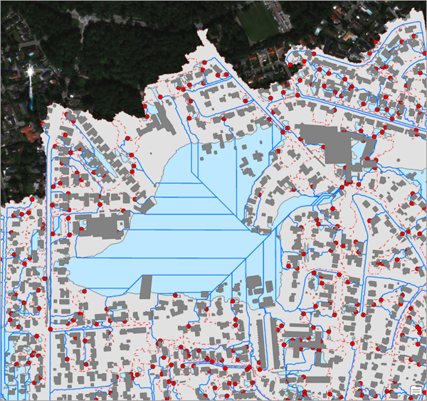
- On the map, zoom in to several smaller bluespots and notice that each detected coherent bluespot has only one pour point and one local watershed. Also, by definition, only one stream carries the spillover from a bluespot when spilling over.
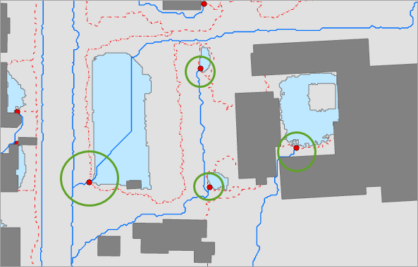
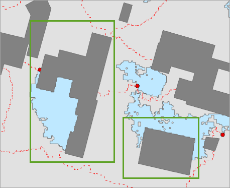
In addition, notice that some buildings seem to be located critically within or next to bluespots—especially if located where outdoor staircases lead into their basements.
- In the Contents pane, uncheck the Bluespots and BluespotWatersheds layers and check the BSDepths layer.
- If necessary, use the Huge Bluespot bookmark.
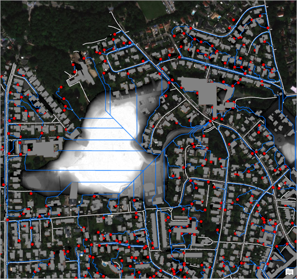
The symbology for the BSDepths layer does not clearly allow you to observe a bluespot’s depth when filled to their pour points. Next, you will modify the symbology of the layer to make this easier to observe.
- In the Contents pane, expand the BSDepths layer.
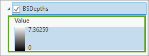
Notice the current layer symbology is a stretch applying grayscale values for the depth range from 0 to 7.3 meters.
Update layer symbology
To update the symbology of layers, complete the following steps:
- In the Contents pane, right-click the BSDepths layer, then choose Symbology.
- In the Symbology pane, click the Primary symbology drop-down menu and choose Classify.
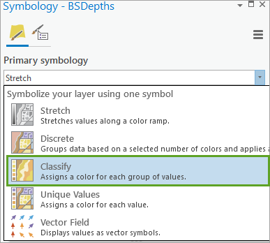
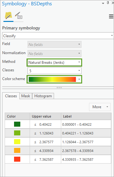
The default classification method is the Natural Breaks (Jenks) method with 5 classes. For this layer, this method will allow you to easily observe bluespot depths.
- In the Symbology pane, click the Color scheme drop-down menu and choose a continuous scheme going from green to red.
- In the Symbology pane, click the Advanced symbology options button.
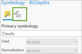
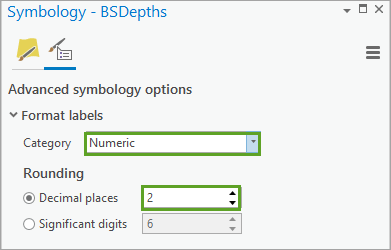
- In the Symbology pane, for Advanced symbology options, expand Format labels.
- For Category, verify Numeric is selected, then for Decimal places, type 2.
- When done, close the Symbology pane.
- In the Contents pane, review the BSDepths layer.
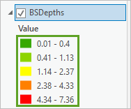
Different bluespot depths are now easier to differentiate; some of them are very deep—up to approximately 7 meters—and others are quite shallow.
- In the Contents pane, uncheck the Streams layer.
- In the Map, explore the BSDepths layer.
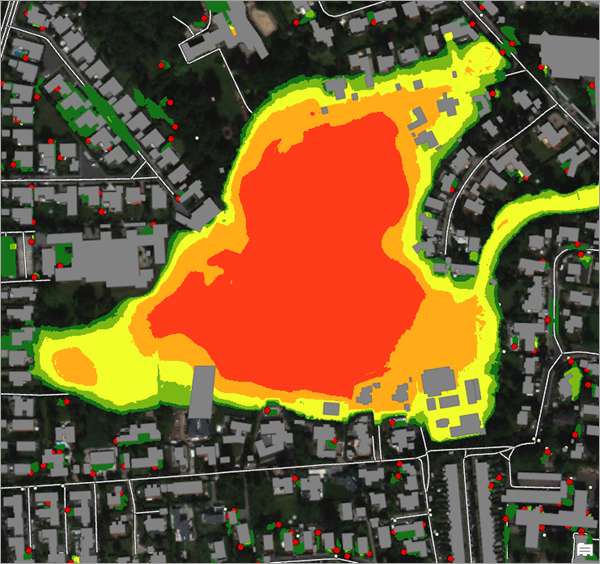
Notice that when a bluespot is filled to its pour point, it is visible. In addition, the depth map includes all minor bluespots that were ignored by the threshold setting because they were shallower than 0.05 meters (5 cm) and had volumes < 1 m3. So, only the bluespots having a red pour point are preserved.
Investigate attributes
To examine bluespot attributes, complete the following steps:
- In the Contents pane, check the Bluespots layer, right-click it, and choose Attribute Table.
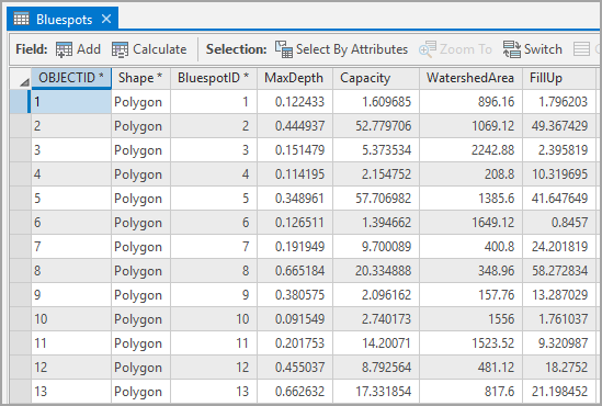
The table indicates that the study area has 3,388 preserved bluespots.
Note:
You may need to scroll to the bottom of the table to load all records to determine the total number of bluespots.
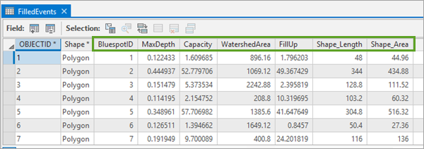
- Review the Bluespot attribute table fields:
- There is a unique BluespotID for each feature
- Notice the asterisk after some field names indicating that the field is indexed to speed up performance when establishing joins later
- The maximum depth (in meters)
- The capacity (in m3) when filled to the pour point level
- The local contributing watershed area (in m2)
- The FillUp value (in mm), which is the ratio of a bluespot’s capacity in m3 versus its watershed area in m2 multiplied by 1,000. This value indicates the amount of precipitation required to fill up a bluespot to its pour point level when assuming 100 percent surface runoff and no contributions from upstream spillovers.
Meanwhile, this ratio may not be as significant, as bluespots having small capacities but relatively large local watersheds (such as the first occurrence in the table) will fill up even at very small rain events. Which is, of course, only the case if the surface is totally impervious (which is part of the assumptions when using this screening method).
- In the Contents pane, drag the BSDepths layer below the Bluespots layer.
- If necessary, use the Huge Bluespot bookmark to zoom to the extent where the largest bluespot is located.
- On the ribbon, on the Map tab, in the Navigate group, click the Explore tool.
- Using the Explore tool, click the large bluespot, then review the Pop-up.
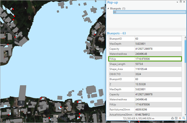
Notice its FillUp value is 1716.978506 mm and it has a very high Capacity (412927.286978) versus its local WatershedArea (240496.48).
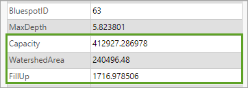
This means that this bluespot will never get filled up by water coming from only its local watershed, since rainstorms of such magnitude (fortunately) never occur in Denmark. Meanwhile, this bluespot may have contributions from other upstream bluespots spilling over, and that is what you are going to investigate later.
- Close the Bluespot layers attribute table and the Pop-up.
- In the Contents pane, right-click the PourPoints layer, then choose Attribute Table.
The PourPoints layer contains attribute fields joined from the Bluespots layer.
- Review the PourPoints attribute table fields.
- Each Pour Point is identified by its BluespotID.
- The Z field has information on the pour points elevation.
- The Capacity (in m3) of the bluespot.
- The pour points contributing WatershedArea (in m2)
- The FillUp value (in mm) is the ratio of a bluespots capacity in m3 versus its watershed area in m2 multiplied by 1,000.
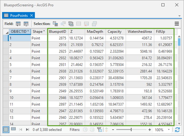
Since the PourPoints layer carries the necessary quantitative information needed to model the downstream spillovers from the bluespots, you will use this layer to model the downstream spillovers from the bluespots at various rain events.
- Close the PourPoints attribute table.
The last output from the model you will review is the Streams layer.
Explore streams
To review streams, complete the following steps:
- In the Contents pane, check the Streams layer, then drag and position it above the Bluespots layer.
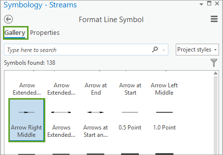
- Expand the Streams layer and double-click the blue line symbol to display the Symbology pane.
- In the Symbology pane, click Gallery.
- In the Gallery, choose the Arrow Right Middle symbol.
- In the Symbology pane, click Properties, then click the Layers button.
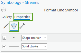
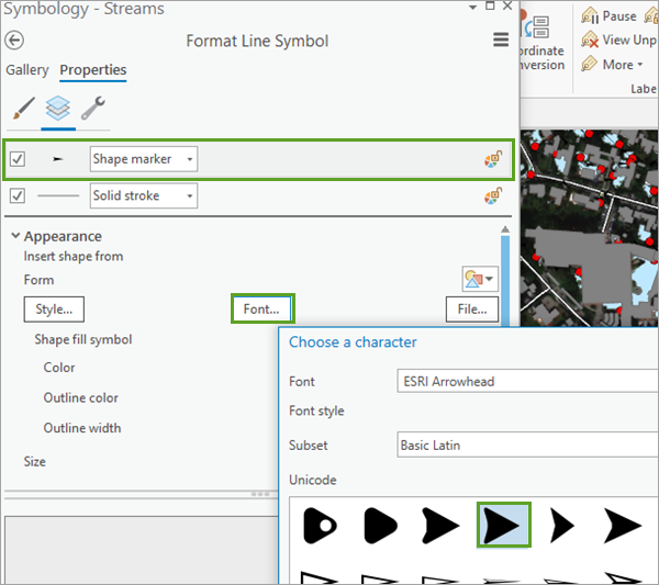
- Click and select Shape marker, then click the Font button.
- In the Choose a character window, choose a suitable arrowhead character, then click OK.
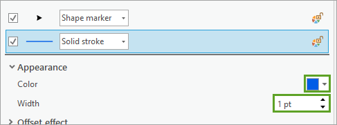
- Click and select Solid stroke, then expand Appearance and modify Color to dark blue and set Width to 1 pt.
- In the Symbology pane, click Apply.
- In the Contents pane, uncheck the BuildingsNoGaps layer.
- In the Contents pane, check the Bluespots, PourPoints, and Streams layers.
- Use the Inspection of nodes bookmark to review PourPoints, Bluespots, and Streams.
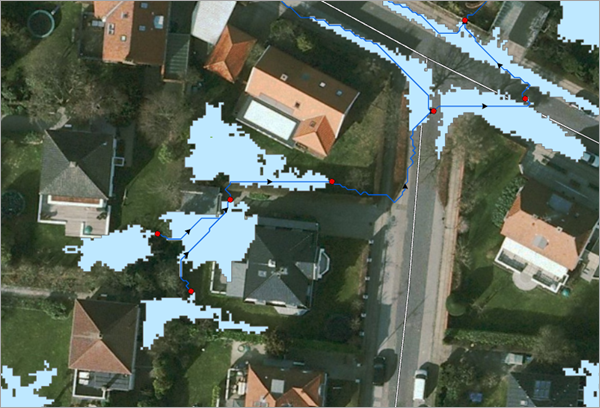
Now the stream flow directions should be easy to inspect on the map. Arrows indicate the downstream flow from a bluespot to the next lower lying bluespot.
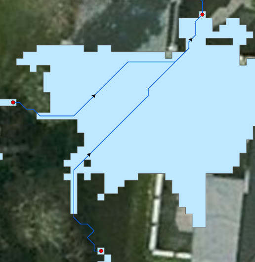
While reviewing this map subset, imagine the complexity of the total stream network, and how tedious it may be to calculate the accumulated spillover from one bluespot to the next ones downstream for the entire study area.
- Click Save to save the project.
Create nodes and edges
This step prepares the hydrologic network to trace the accumulated downstream spillover from the bluespots pour points along the detected flow paths, representing your derived streams.
To enable tracing, the network's topology must be built to define its connectivity. The pour points define the starting points for the streams in the network, but it is also necessary to know the endpoints for all line features. If a stream goes from one pour point straight into another bluespot downstream, the stream line feature ends at its pour point, and everything is fine. But when two streams intersect, you must consider the establishment of a new node located at the junction as part of the hydrologic network.
- In the Catalog pane, expand Toolboxes, and expand BluespotScreening.tbx.
- Double-click the Create Nodes and Edges script tool.
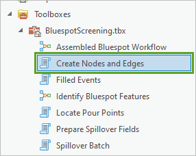
- In the Create Nodes and Edges tool, update the following parameters:
- For Input PourPoints Feature Layer, choose PourPoints.
- For Input Streams Feature Layer, choose Streams.
- For Output Workspace, choose your Outputs.gdb geodatabase.
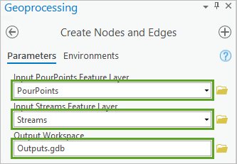
- Click Run.
In the Create Nodes and Edges tool, you may want to display the Results messages.
Note that there are still 3,388 true pour points, but 2,007 new junction nodes were added to the end of the attribute table.
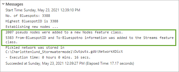
When building the hydrologic network, the junction nodes are simply added to the pour point nodes in a Nodes feature class, where the node IDs match the corresponding BluespotIDs.
- In the Contents pane, verify the Nodes layer was added. If not, locate and add the layer from your Outputs.gdb geodatabase.
- In the Contents pane, expand the Nodes layer, then double-click the point symbol. In the Symbology pane, modify the symbol color to green.
- If necessary, check and drag the Nodes layer above the Streams layer.
- In the Contents pane, right-click the Nodes layer and choose Label.
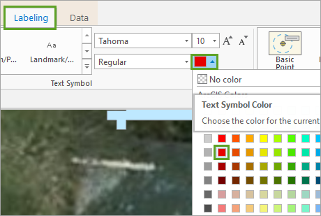
- On the ribbon, on the Label tab, in the Text Symbol group, click the Text Symbol Color button and choose red.
Use the Inspection of nodes bookmark to zoom to the extent of several small bluespots. If necessary, zoom in closer to inspect.
The red nodes are pour point nodes and the green ones are junction nodes located where streams intersect.
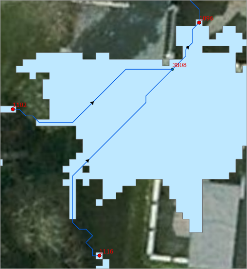
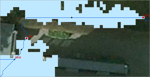
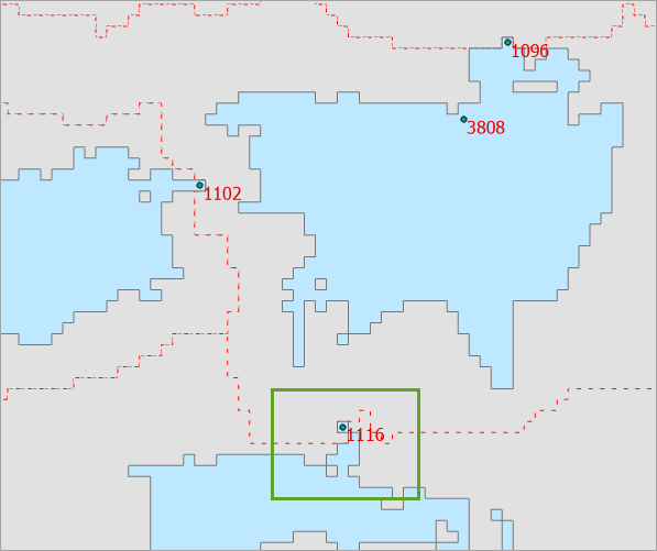
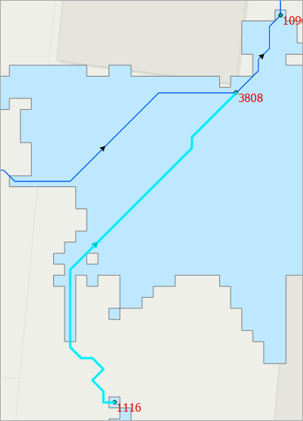
Notice how one stream in the south originates at the pour point with BluespotID 1116, and another stream in the west originates at the pour point with BluespotID 1102. Both streams end where they merge at the junction node with BluespotID 3808. From there, a new stream begins and ends at the pour point with BluespotID 1096, where a new stream begins and ends at the pour point with BluespotID 1079.
Note:
To estimate the water volumes going downstream from the pour point nodes, through the junction nodes at different rain events, you use a hierarchical network and then consider capacities and volumes captured at each pour point.
- On the ribbon, on the Map tab, in the Selection group, use the Select tool to select the PourPoints, Steams, and Nodes that form a subset of features on the map.

Ensure the Streams, PourPoints, and Nodes are selected.
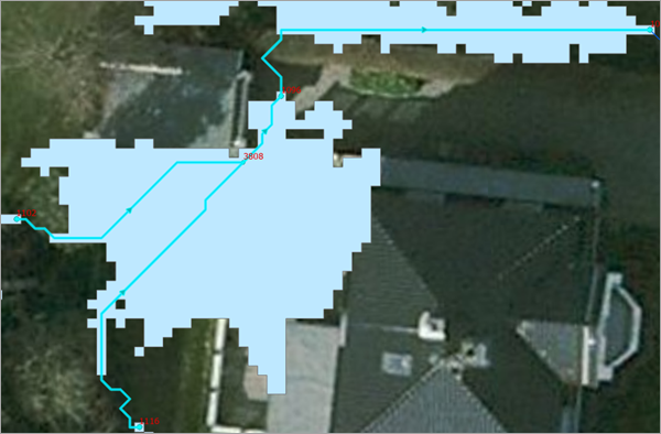
- In the Contents pane, right-click the Nodes layer and choose Attribute table.
- Review the Nodes attribute table.
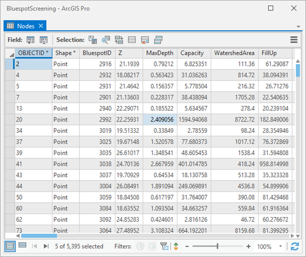
As you scroll records in the table, you may notice the missing values <Null> for MaxDepth, Capacity, WatershedArea, and FillUp for the junction nodes. You will explore these later.
- In the lower left of the Nodes table, click the Show selected records button.
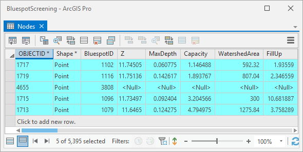
Note:
Your hydrologic network contains stream topology generated using the networkx Python package. This file should be saved in the project's home folder, however, for this lesson, the binary file containing the stream networks topology, which is named NetworkXDict, is saved in the Outputs.gdb geodatabase for fast retrieval when generating the SpillOverBatch. It contains a Python dictionary where the keys are a combination of each individual stream's start and end nodes, and its corresponding value is the stream's OBJECTID
. - In the Contents pane, right-click the Streams layer and choose Attribute table.
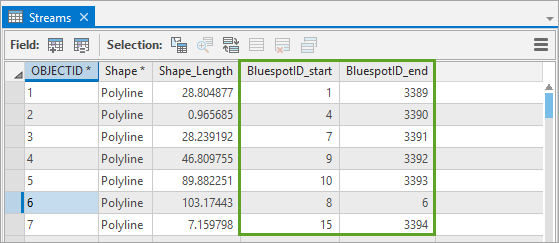
- Review the Streams attribute table.
Notice that the Streams attributes include a BluespotID_start and BluespotID_end field.
- In the lower left of the Streams table, click the Show selected records button.
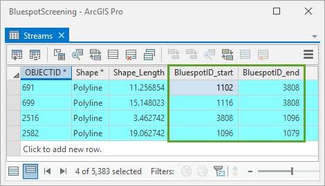
You can now observe the sequence of flow from BluespotID 1116, and 1102, into 3808 and from 3808 into 1096 and then 1079.
- Close the Nodes and Streams attribute tables.
Note:
When a process accesses a dataset, it locks the dataset, preventing other processes from modifying it. When the process terminates, the lock files associated with it are automatically deleted. Viewing and selecting records in the nodes and streams table has caused them to be locked, thus by closing the tables you remove the locks and thereby allow records in the tables to be updated in future steps.
- On the quick access toolbar, click Save to save the project.
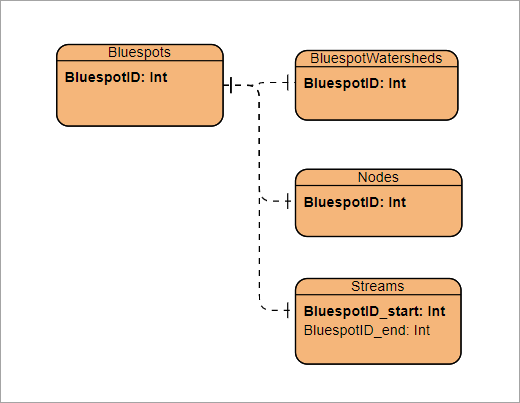
Now the data modeling is complete. Before continuing, review the one-to-one relationships established in the model.
Prepare spillover fields
Having configured the basic hydrologic network, including the bluespots, their pour points, the junction nodes, and the streams connecting them, we are almost ready to determine the results of various storm water scenarios in our study area. The only thing remaining is to predefine a series of uniform rain events that will be used in the next spillover calculations.
The Prepare Spillover Fields script tool adds a number of extra fields for each rain event to the Nodes feature class to keep track of incoming and outgoing volumes for each bluespot. Of course, it is recommended that you establish realistic storm water scenarios matching your area of interest. So, for the Charlottenlund region, rain event scenarios ranging from 20 to 100 mm in steps of 10 mm are considered, as these realistically reflect events occurring annually in the area versus those occurring only once in a thousand years (approximately).
Note:
It is also possible to simulate the spillover at nonuniform rain events, as the water volumes added to the individual bluespots’ watersheds might be assigned individually. This was done in a study of the effects of local snowmelt in Greenland. Review this research paper for more details.
- In the Catalog pane, expand BluespotScreening.tbx
- Double-click the Prepare Spillover Fields script tool.
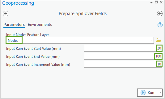
The only parameters required are the names of the Input Nodes Feature Layer or Feature Class that you created in the previous modeling steps and the Input Rain Event Start Value, the End Value, and the Increment Value in millimeters.
- In the Prepare Spillover Fields tool, update the following parameters:
- For Input Nodes Feature Layer, choose Nodes.
- For Input Rain Event Start Value (mm), type 20.
- For Input Rain Event End Value (mm), type 100.
- For Input Rain Event Increment Value (mm), type 10.
- Click Run.
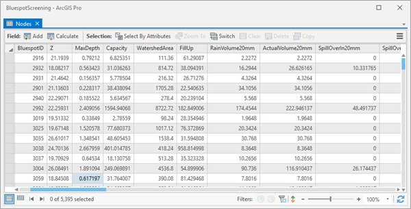
- When complete, open the Nodes feature class attribute table.
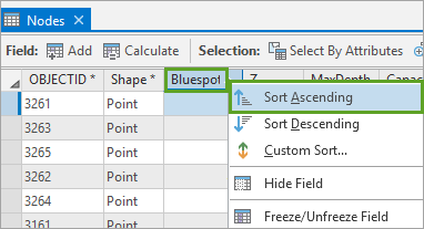
- In the Nodes table, right-click the Bluespot field, then choose Sort Ascending.
- Review the Nodes attribute table fields, and locate the first record where the Bluespot value equals 1.
- Review the RainVolume20mm field.

The RainVolume20mm field contains the rain volume entering a bluespot from its local catchment (watershed) at a specific rain event. When looking at the table, the RainVolume20mm is calculated as 20 mm of precipitation times the WatershedArea 896.16 m2 = 17.9232 m3.
- In the Nodes table, clear any selections.
- Close the Nodes attribute table to remove locks
- Save the project.
Spillover Batch
Next you will use the Spillover Batch script tool to calculate the downstream accumulated spillover from one bluespot to the next bluespot or bluespots downstream.
The tool loads the stream network topology saved in the NetworkXDict file. Graph theory identifies this type of network as an acyclic directed graph. This means that it is a network, ordered hierarchically and having one direction only, which is downstream. Such a network cannot have loops, thus if the tool returns an error, it may be due to a stream diverting and then re-merging. As a result, this screening method is not applicable in totally flat areas, dominated by meltwater plains (sandurs), as found in Iceland or in flat-diked areas on marshland.
- In the Catalog pane, expand BluespotScreening.tbx.
- Double-click the Spillover Batch script tool.
- In the Spillover Batch tool, for Input Nodes Feature Layer, click browser and navigate to the Output.gdb and choose Nodes.
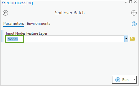
- Click Run.
During the execution, you can monitor the output messages in the View Details pane (see below). Notice the very fast processing time.
Note:
To understand the sequence for the spillover calculations, review the following article on spillover engine.
- Use the Inspection of nodes bookmark to update the map extent.
- In the Contents pane, right-click the Nodes layer and click Attribute Table.
The table contains four fields for each of the nine rain events examined, in other words, 36 fields.
- In the Nodes table, click the far right of the first record, then right-click and choose Pop-up.
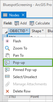
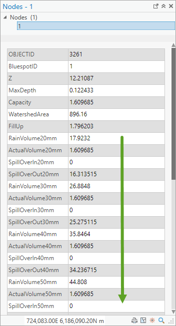
The pop-up appears and it is easier to review the four fields generated for each of the nine rain events examined, in other words, 36 fields.
- Spend a few minutes investigating the calculated downstream accumulated spill for the various rain event scenarios ranging from 20 to 100 mm in steps of 10 mm.
- Close the Pop-up when you are done.
- In the Nodes table window, click the Select by Attributes button.
- In the Expression builder, create the following expression:
- For Field Name, choose BluespotID.
- For Operator, choose includes the value(s).
- For Values, type 1079,1096,1102,1116,3808.
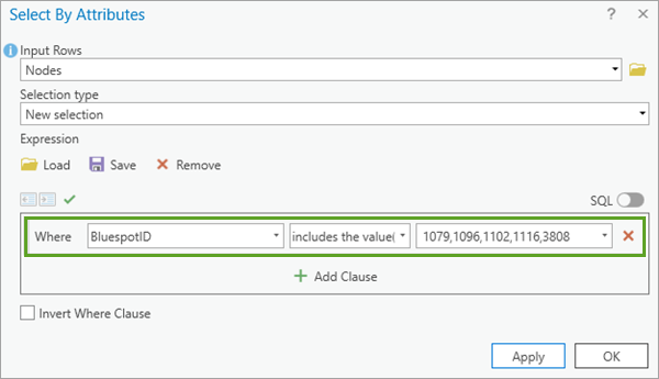
- Verify the expression and click Apply.
- Click OK to close the Select By Attributes pane.
- In the Nodes attribute table, click the Show selected records button.
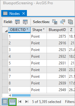
The table updates and filters to show only selected records. If necessary, expand the table to review additional fields.

This table contains four fields for each of the rain events examined. For each of them, the balance for each bluespot based on values stored in the Nodes feature class can be derived as follows:
SpillOverOut = SpillOverIn + RainVolume – Capacity
So, for the 20 mm rain event, you need to consider the balance obtained from these fields:
SpillOverOut20mm = SpillOverIn20mm + RainVolume20mm – Capacity
To get the results right, you start at the beginning of a local network and look at all values rounded to three decimals—for example, at the node with BluespotID 1116 that has a Capacity of 1.894 m3.

At a 20 mm rain event, the incoming rain volume from its surrounding local watershed saved in the RainVolume20mm field is 16.141 m3. As this bluespot has no upstream contribution, the SpillOverIn20mm field is 0, so the SpillOverOut20mm field is calculated as 16.141 - 1.894 m3 = 14.247 m3.
Next, explore the balance for the node with BluespotID 1102. The balance here sums to 10.700 m3.

Now, as the spillover for the nodes with BluespotID 1102 and 1116 merges at the junction node with BluespotID 3808, the junction node’s balance is totaled from a sum of the incoming spillovers from the nodes with BluespotID 1102 and 1116, only, as this node doesn’t have any contributing watershed. Thus, the balance at BluespotID 3808 is 24.947 m3.

Next, the balance at the node with BluespotID 1096 is 24.947 + 6 – 3.205 m3 = 27.742 m3.

This example demonstrates how the balances are worked out hierarchically, first considering the farthest upstream bluespots. Then the calculations go deeper and deeper into the network until the calculations end at the drainage basin’s terminal point located at the outlet into the sea.
- In the Nodes table, click the Clear button to unselect records.
- In the Nodes table, click the SpillOverOut20mm field, then choose Sort Ascending.
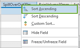
Notice that several bluespots don’t produce spillovers because of their large capacities.
- When you are done, clear any selections and close the table.Calculating downstream accumulated spillover from one bluespot to the next bluespot or bluespots downstream
To understand the sequence for the spillover calculations, review the figure below or read the scientific article on spillover engine .
In the illustration, the topological setup of streams and nodes is visualized. Bluespots are represented by nodes, A-G, and streams as black edges going from one node to the next downstream. For each bluespot, the values xx/yy represent volumetric contributions from a bluespot’s local catchment (xx) versus its capacity (yy).
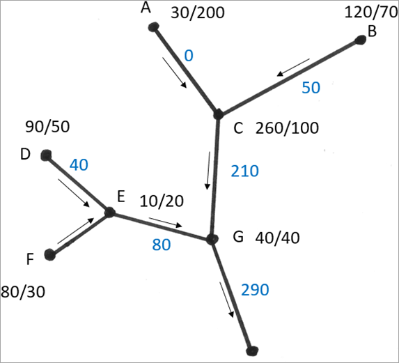
Node A represents a bluespot with a capacity of 200 volumetric units, but the bluespot's local catchment contributes with 30 units only, resulting in no spillover along the edge toward the bluespot at node C. The bluespot at node B has a capacity of 70 but at a delivery of 120 volumetric units from its local catchment. Thus, 50 units of spillover is transported downstream to the bluespot represented by node C. That bluespot has a capacity of 100, but 260 units are supplied from its local catchment, providing a spillover of 160 units. Moreover, 0+50 units must be added from upstream spillover at node A and B entering C, resulting in a total of 50 + 160 = 210 units transported toward node G. However, the water balance for that bluespot must await the results from the spillover at junctions D, E, and F before it can be estimated and so forth.
According to a stream order classification method by Strahler, edges AC, BC, DE, and FE are first order streams. When two first order streams merge, they become second order streams such as edges CG, EG, and so forth. Thus, the network shown is a third order Strahler stream network, and the bluespots appearing at the beginning of the network are named first order bluespots.
When looking into the associated script’s Python code (which can be done by right-clicking the script tool’s name in the BluespotScreening toolbox and selecting Edit), the structure necessary for defining the acyclic graph is very basic. First, an acyclic directed graph, G, is defined and populated by all stream polylines as edges and all their start and endpoints as nodes. When generated, the network is stored in the NetworkXDict file for easy retrieval when spillovers are calculated for many rain events.
Next, the network's nodes are sorted topologically and saved in a list, so when stepping through it, all nodes and edges are stored (and retrieved) in exactly the right hierarchical sequence in accordance with the topological setup described previously. Thus, all so-called first order nodes and edges appear first in the list, then the second order ones, and so on. In that way, the network is ready to trace the hierarchical downstream spillovers.
Filled Events
The final analysis step is an extension of the previous steps in which you were investigating the rain event at which the bluespot starts spilling over. After calculating downstream accumulated spillover, you can look up the smallest rain event producing a spillover from a bluespot by reviewing the SpillOverOutxxxmm fields in the Nodes attribute table.
This is done by searching for a value > 0 and saving the matching rain event in a new field named FilledEventmm. If no spillover is observed (if a bluespot has a huge capacity not being filled up at the most extreme rain event investigated), a field value of -1 is assigned.
- In the Catalog pane, locate and expand BluespotScreening.tbx.
- Double-click the Filled Events script tool.
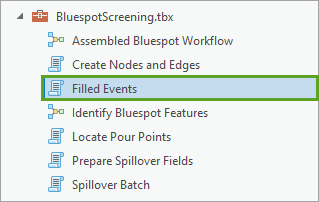
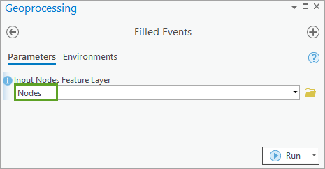
The Filled Events tool requires the Nodes feature class as input.
- In the Filled Events tool pane, for Input Nodes Feature layer, choose Nodes.
- Click Run.
- Display the Nodes attribute table.
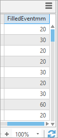
- In the Nodes table, review the FilledEventmm field values.
The values represent the rain event at which the bluespot starts spilling over.
- In the Nodes table, click the FilledEventmm field, then choose Sort Ascending.
Notice that several bluespots are assigned a field value of -1. These bluespots have a huge capacity and do not fill up, even at the at the most extreme rain events investigated.
- Close the Nodes table and click Save to save the project.
In this module, you reviewed and explored a sample dataset and used the tools (models and scripts) to predict the flooding consequences from a series of simulated storm water events. In the next module, you will evaluate and interpret the results of the bluespot modeling. The additional fields populated by the Filled Events tool will form part of this interpretation.
Next, you will assess the modeling outputs and gain a better understanding of storm water consequences at different storm scenarios. The goal is to predict the overall consequences of storm water to various societies and consider where to avoid future site developments without taking the necessary precautions in times of climate changes. The predictions are based on the screening of a digital terrain model for landscape depressions within a drainage basin, their hierarchical downstream locations, and how they will be filled up and spill over during simulated uniform rainstorms neglecting local infiltration rates and time.
Explore the results
In this module, you will inspect the results generated by the Identify Bluespot Features model and the additional tools you used to create nodes and edges and calculate downstream accumulated spillover from one bluespot to the next bluespot or bluespots downstream. You will evaluate model outcomes to explore the consequences of storm water within the study area. A broader goal is to predict the overall consequences of storm water to the study area and consider where to avoid future site developments that will be impacted adversely by climate changes.
Explore Bluespots, BluespotWatersheds, Nodes, and Stream features
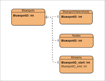
To facilitate exploration of the model results, you will need to finalize data processing by attaching nodes feature attributes to the Bluespots, Streams and BluespotWatersheds features. This will be achieved by joining and building one-to-one relationships for features with matching IDs.
The illustration below describes the one-to-one relationships and the matching ID fields.
- If necessary, open the BluespotScreening project.
Before you continue, you will add a new map to your project and copy only the necessary layers needed for interpretation.
- On the ribbon, on the Insert tab, in the Project group, click the New Map button.
A new map named Map1 is added to the project. You will use this map to investigate and explore the consequences of storm water in the Charlottenlund study area.
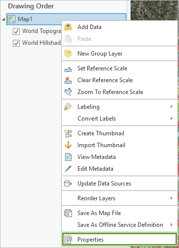
- In the Contents pane, right-click Map1, then choose Properties.
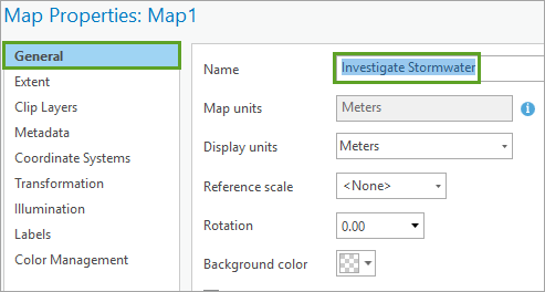
- In the Map Properties pane, on the General tab, for Name, type Investigate Stormwater. Click OK to close the Map Properties pane.
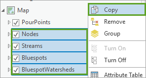
- In the project, in the Contents pane of Map, check Nodes, Streams, Bluespots, and BluespotWatersheds, then right-click and choose Copy.
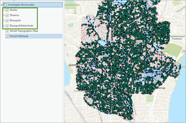
- In the Investigate Stormwater map, in the Contents pane, right-click Investigate Stormwater and choose Paste.

The selected layers are duplicated in the Investigate Stormwater map.
- In the Contents pane, right-click Investigate Stormwater, then click Reorder Layers and choose By Type.
This will ensure point and line layers are displayed above polygon layers.
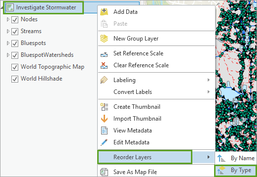
- On the ribbon, on the Map tab, in the Navigate group, use the Inspection of Nodes bookmark to zoom to a series of connected bluespots.
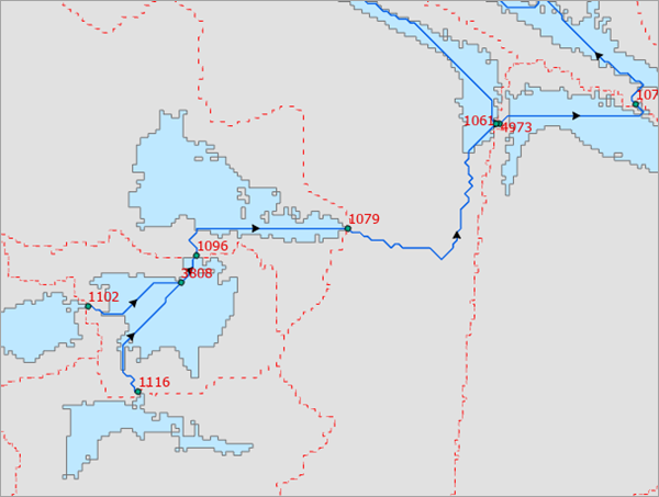
- Nodes may already be labeled; if not, in the Contents pane, right-click the Nodes layer and choose Label
- In the Contents pane, click on Nodes layer to activate it.
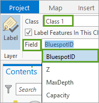
- On the ribbon, click the Labeling tab.

- On the Labeling tab, in the Label Class group, for Class 1, for Field, verify BluespotID is selected.
- On the Labeling tab, in the Text Symbol group, verify Font is set to Tahoma and Size is set to 12.

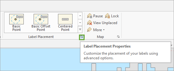
- On the Labeling tab, in the Label Placement group, click the Label Placement Properties button.
- In the Label Class – Nodes pane, for Placement, choose Bottom right of point.
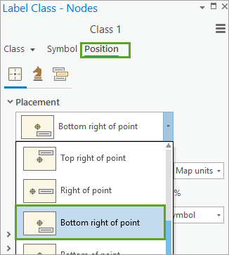
Labels are now placed at the lower right of the node point and are easily readable.
- Close the Label Class – Nodes pane.
- In the Contents pane, uncheck the Streams layer.
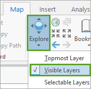
- On the ribbon, on the Map tab, in the Navigate group, click the drop-down menu for the Explore tool and choose Visible Layers.
- On the map, zoom in to the bluespot where the node has a BluespotID equal to 1116.
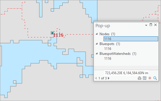
- Click the node labeled 1116 and review the pop-up.
Notice that both the Bluespots and the BluespotWatersheds features have matching IDs = 1116.
- In the Contents pane, check the Streams layer and uncheck the BluespotWatersheds layer.
- On the ribbon, on the Map tab, in the Selection group, choose the Select tool.
- On the map, select the stream leaving the node with BluespotID equal to 1116.
- In the Contents pane, right-click Streams, then choose Attribute Table.
- In the Streams attribute table, click the Show selected records button and review the attributes of the selected stream.
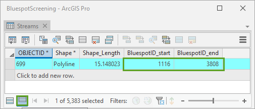
Notice that the selected stream starts at the bluespot with ID value 1116 and ends at the bluespot with ID value 3808.
Since the BluespotID values are available and serve as a key field, you can transfer results in the Nodes layer to the Bluespots and Streams layers through joins.
- Clear the selected Streams feature and close the Streams attribute table.
- In the Contents pane, right-click the Nodes layer and choose Label.
This will remove node labels from the map.
- Save the project.
Investigate filled events and buildings layer intersections
Next, you will visualize the events at which a bluespot starts spilling over, by joining nodes layer attributes to the Bluespots layer.
- In the Investigate Stormwater map, in the Contents pane, right-click the Bluespots layer and choose Copy, then right-click Investigate Stormwater and choose Paste.
The Bluespots layer is duplicated in the Contents pane. Next, you will rename the copy of the layer.
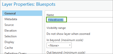
- In the Contents pane, right-click the copy of the Bluespots layer and choose Properties.
- In the Properties pane, for Name, type FilledEvents, then click OK.
- In the Contents pane, right-click the FilledEvents layer, then choose Attribute Table.
- Review the attribute fields in the FilledEvents attribute table.
- When done, close the FilledEvents attribute table.
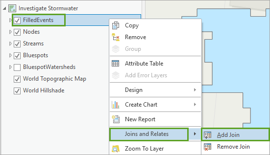
- In the Contents pane, right-click the FilledEvents layer, hover over Joins and Relates and choose Add Join.
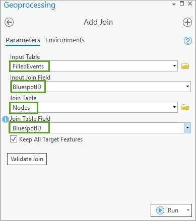
- In the Add Join tool, update the following parameters:
- For Input Table, verify FilledEvents is selected.
- For Input Join Field, choose BluespotID.
- For Join Table, choose Nodes,
- For Join Table Field, choose BluespotID.
- Verify all tool parameters and click Run.
- In the Contents pane, right-click the FilledEvents layer, then choose Attribute Table.
- Review the joined attribute fields in the FilledEvents attribute table. Close the table when done.
Notice the addition of the storm water event modeling attributes originally contained in the Nodes layer.

Update layer symbology
To update the symbology of layers, complete the following steps:
- In the Contents pane, right-click FilledEvents, then choose Symbology.
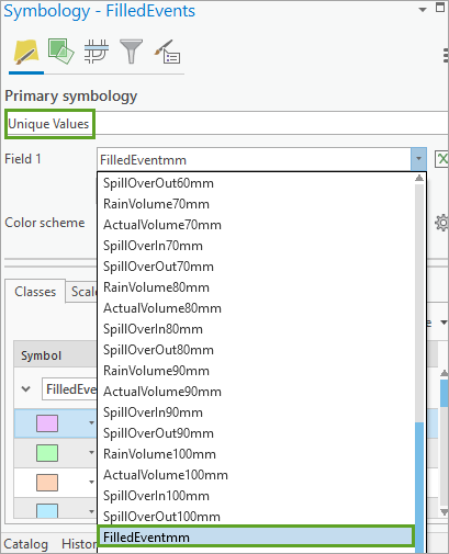
- In the Symbology pane, click the Primary symbology drop-down menu and choose Unique Values.
- For Field1, click the drop-down menu and choose the FilledEventmm field.
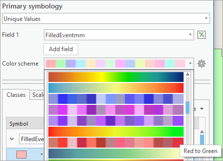
- In the Symbology pane, click the Color scheme. In drop-down menu, check on Show all and choose a continuous scheme going from Red to Green.
- On the Classes tab, double-click the red color symbol for the -1 entry.
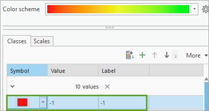
The Symbology pane appears.
- In the Properties tab, under Appearance, for Color, click the color drop-down menu and choose a gray color. Click Apply.
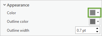
- Click the Return to primary symbology button.
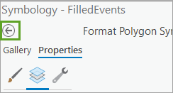
- On the Classes tab, double-click the orange color symbol for the 20 entry.
- In the Appearance pane, for Color, click the color drop-down menu and choose red. Click Apply and then click the Return to primary symbology button.
- Verify the updated colors and close the Symbology pane.
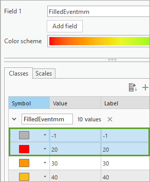
- On the map, zoom to the extent of the study area and explore the updated symbology.
All filled events or bluespots are now symbolized according to the rain event where the incoming water volume exceeds a bluespot’s capacity, so the color represents the rain event at which a spillover begins to take place.
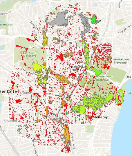
This also means that the bluespots spilling over have reached their maximum filled horizontal extent. All sinks symbolized in gray have such high capacities that they are not yet filled and will not spill over even at the biggest rain event modeled—in this case, the 100 mm event.
Next, you will use a chart to visualize filled events.
Create a chart
Charts give you an opportunity to summarize and visualize filled events in a concise and simple manner.
- In the Contents pane, select the FilledEvents layer.
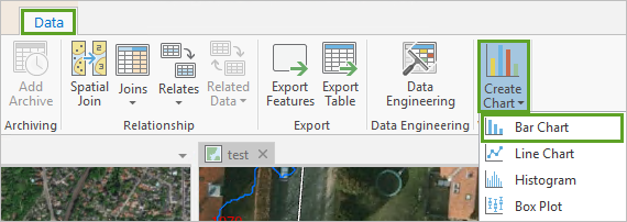
- On the ribbon, click the Data tab. In the Visualize group, click the Create Chart drop-down menu and choose Bar Chart.
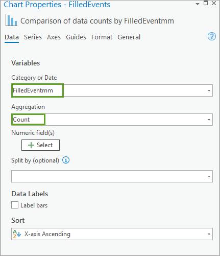
- In the Chart Properties – FilledEvents pane, set the following parameters:
- For Category or Date, choose FilledEventmm.
- For Aggregation, verify Count is selected.
- If necessary, resize and position the Comparison of data counts by FilledEventmm chart, then review the chart content.
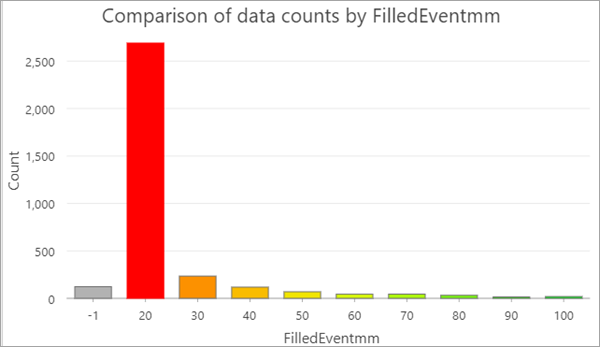
The chart shows the number of bluespots that are filled at a specific rain event (in mm) and start spilling over. Notice that the number of bluespots versus the FilledEventmm decreases asymptotically with increasing rain events.
On the map, notice the large bluespot located east in the study area will not spill over at a 100 mm rain event, either. But looking into its attributes, notice its ActualVolume100mm being 44,845 m3, which is very close to its capacity (45,150 m3). So, presumably, this bluespot will be filled entirely and start spilling over at a 110 mm event.
- In the chart, click the 20 mm bar chart column.
When clicking the 20 mm bar chart column, it shows that 2,689 bluespots are filled at that event. Simultaneously, the matching bluespots are highlighted on the map. Typically, such bluespots are shallow, have small volumes, and are found in gardens and along infrastructures.
- Click the bar with a value of -1.
The map and chart identify 126 bluespots. When zooming in to them, most are located as first order bluespots with FillUp values > 100 mm. Meanwhile, some are also located downstream, but have such large capacities that they don’t spill over even at the maximum rain event investigated.
- Explore the bluespot at the bookmark named Huge Bluespot. Click inside the bluespot.
Notice its capacity of 412,927 m3. When reviewing its attributes, notice that for the 100 mm event, the field named ActualVolume100mm shows that the actual stored water volume is 32,372 m3. Thus, buildings located along this depression’s upper rim will never flood.
- In the Chart Properties – FilledEvents pane, set the following parameters:
- For Category or Date, choose FilledEventmm.
- For Aggregation, choose Sum.
- For Numeric Fields, click +Select and choose Capacity and click Apply.
- Review the updated bar chart showing the Comparison of sum Capacity by FilledEventmm.
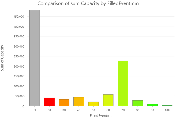
In the chart, notice the bluespots not being filled up at a 100 mm event (still represented by a value of -1) make up the largest summed volume.
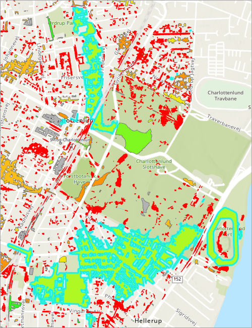
- In the chart, click the 70 mm bar, then review the selected bluespots on the map.
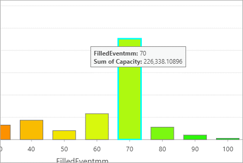
On the map, note that two large bluespots dominate the 70 mm category.
- In the chart, click in a blank space to unselect the 70 mm category.
To estimate how many buildings might be affected during a rainstorm, a selection can be set up for features in the BuildingsNoGaps layer that intersects the filled bluespots at the 70 mm event.
- In the project, in the original Map, in the Contents pane, select the BuildingsNoGaps layer, then right-click and choose Copy.
- In the Investigate Stormwater map, in the Contents pane, right-click Investigate Stormwater and choose Paste.
- On the ribbon, on the Map tab, in the Selection group, click the Select by Attributes tool.
- In the Select By Attributes pane, click New expression.
- For Input Rows, choose FilledEvents.
- In the Expression builder, for Field Name, choose FilledEventmm.
- For Operator, choose is less than or equal to.
- For Value, choose 70.
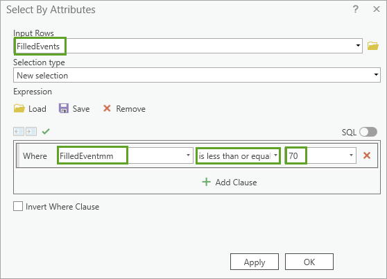
- Verify the expression, then click Apply.
As a result, 3,322 bluespots are selected.
- Click OK to close the Select By Attributes pane.
Next, use the Select By Location tool to identify the BuildingsNoGaps features that overlap the selected filled bluespots.
- On the ribbon, on the Map tab, in the Selection group, click the Select By Location tool.
- In the Select By Location pane, set the following parameters:
- For Input Features, choose BuildingsNoGaps.
- For Relationship, choose Intersect.
- For Selecting Features, choose FilledEvents.
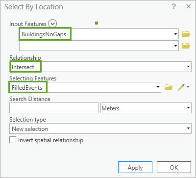
- Verify the parameters, then click Apply.
As a result, 3,126 buildings are selected. This means that 3,126 buildings are affected by bluespots, some more than others depending on their intersecting locations.
- Click OK to close the Select By Attributes pane.
- Save the project.
What can we learn about bluespots and buildings?
This analysis raises several interesting questions concerning a building’s flood risk due to its bluespot adjacency—especially if the bluespot is located next to a building where a staircase leads into the basement. In this case, the flood damage may be more severe than for similarly located buildings without basements. If information about staircase locations were available, the flood risk might be depicted much more accurately when combined with the bluespots’ depths around the staircases.
Another consideration is that buildings located completely within filled bluespots may be at higher risk than others. However, when selecting by location to identify buildings located completely within bluespots, no matches are returned, even if a visual inspection identifies such occurrences. Why is that?
- First, consider that all building footprint polygons have been converted from a vector to a raster format and are burned onto the DTM enforcing runoff around them. Logically, this means that we will never identify bluespots inside buildings.
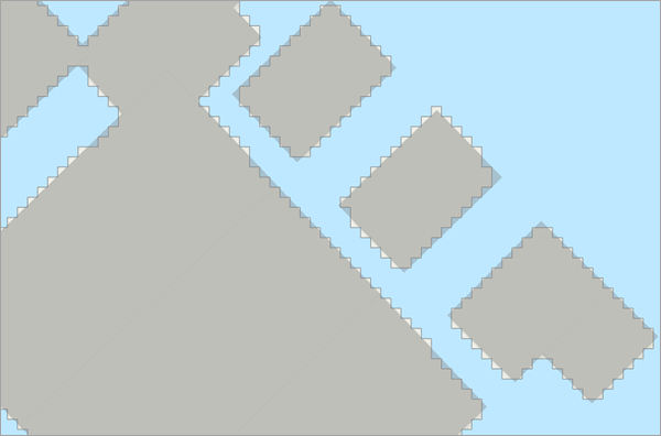
- Second, the derived bluespot areas were originally a raster representation, converted to vector polygons without feature simplification applied.
- In combination, this means that when Select By Location is used on the Bluespots (or FilledEvents) layer using the Intersect spatial relationship, the vectorized bluespots are matched with the BuidlingsNoGaps vector footprints. Thus, overlaps are identified, as shown in the figure below, unless a building is oriented perfectly along the elevation model’s cells. If that is the case, no matches are found. In addition, if Select By Location is used on buildings located Completely Within bluespots, as mentioned before, no matches are identified.
- No matches identified is a limitation related to the data representations, and what was prioritized for the analysis: In this example, the location of buildings and the volumes that they occupy were prioritized over the ability to identify buildings located completely within filled bluespots.
- If you did want to select buildings located completely within bluespots, everything must be remodeled using a DTM without buildings incorporated. This would cause bluespot volumes to be inaccurate, as building volumes are not accounted for affecting bluespot capacity and spillover estimations.
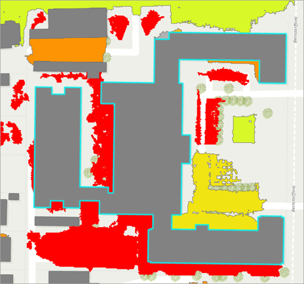
- An additional consideration is that if you try to examine which buildings intersect bluespots at various filled events, some large buildings may intersect bluespots having different filled events. The example below shows a building affecting 20-, 50- and 60-mm events. In this situation, when deriving statistics to count the number of buildings located next to bluespots filled up at various events, the same building may be counted more than once. In these cases, the building should only be counted with the lowest filled event value, which in the example illustrated is 20 mm.
You also need to consider flood risks to buildings located in bluespots at rain events only causing a partial fill-up. In these cases, depth/volume relationships must be considered for the bluespots in question to estimate the water levels matching specific and actual bluespot volumes. As a result, a depth/volume relationship curve must be established for each bluespot incremented, for example, in steps of 5 centimeters depending on the spatial resolution and accuracy of the DTM used. In this way, water depth can be estimated at a given volume.
And lastly, the bluespot’s horizontal and partly filled (shrunken) extent can be depicted and buildings identified that intersected at that level. This analysis requires an additional set of tools that are not currently included in the model but are in consideration for future enhancements to the workflow.
Next, you will map the bluespot spillovers.
Map the bluespot spillovers
The spillover volumes in m3 from a bluespot at a specific rain event indicate how serious the water flow is within it. These values can be visualized like the FilledEvents when the Nodes layer’s attributes are joined onto the Bluespot layer.
- In the Investigate Stormwater map, in the Contents pane, right-click the FilledEvents layer and choose Copy.
The FilledEvents layer is already joined with the Nodes layer; copying the layer will preserve the join.
- In the Contents pane, right-click Investigate Stormwater and choose Paste.
- Rename the new layer to SpillOver60mm.
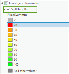
- In the Contents pane, right-click the SpillOver60mm layer, then choose Symbology.
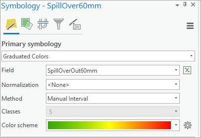
- In the Symbology pane, click the Primary symbology drop-down menu and choose Graduated Colors.
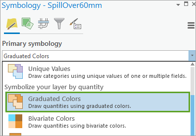
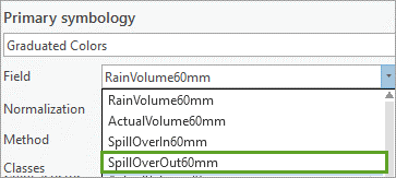
- For Field, click the drop-down menu and choose the SpillOverOut60mm field.
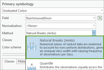
- For Method, click the drop-down menu and choose Natural Breaks (Jenks).
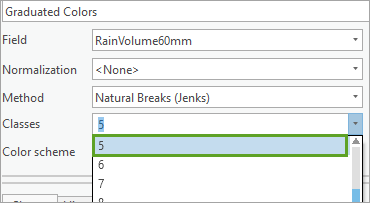
- For Classes, choose 5.
- In the Symbology pane, click the Color scheme drop-down menu and check Show names.
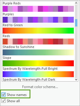
- Choose a continuous color scheme from green to yellow to red.
- In the Symbology pane, click the Advanced Symbology Options button.

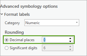
- In Advanced symbology options, locate Format labels and Rounding. Set the number of Decimal places to 0.
- In the Symbology pane, click the Primary Symbology button.

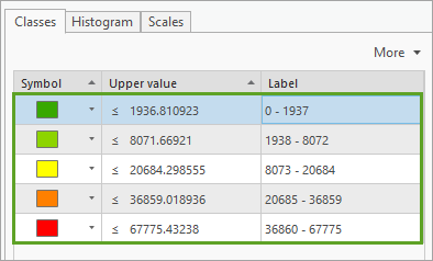
- On the Classes tab, verify the updated layer symbology and rounded labels.
- On the map, zoom to the extent of the study area and explore the updated symbology.
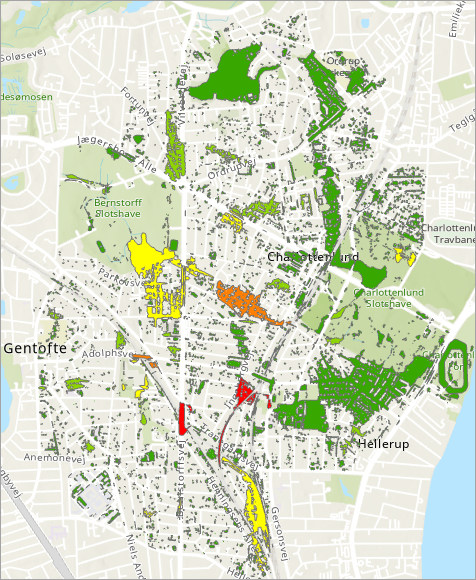
- Use the bookmarks to explore the 60 mm bluespot spillover layer on the map.
- Save the project when done.
What did we learn about 60mm bluespot spillovers?
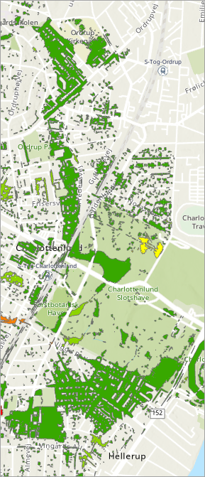
In general, the 60mm spillover is limited in the outskirts of the drainage basin, but as the bluespots overall don’t have capacities that can match the incoming volumes at high rain events, the runoff increases dramatically.
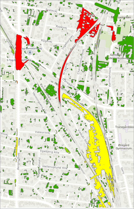
It seems like the volumes in m3 going downstream reach quite high values, especially in the lower central part of the study area next to or overlapping some vital infrastructure.
This is, indeed, critical along the roads toward the southwest that serve a large regional hospital (Gentofte Sygehus).
In the next step, you will investigate how these spillovers may be assigned from bluespots to the flow paths leaving them.
Map the stream spillovers using graduated colors and graduated symbols
The volumes carried along the streams from the bluespots’ pour points can be visualized by joining the Nodes layer's attributes onto the Streams layer.
- In the Investigate Stormwater map, in the Contents pane, right-click the Streams layer and choose Copy.
- In the Contents pane, right-click Investigate Stormwater and choose Paste.
- Rename the new layer to StreamVolumes.
- In the Contents pane, right-click the StreamVolumes layer, hover over Joins and Relates and choose Add Join.
- In the Add Join tool, update the following parameters:
- For Input Table, verify StreamVolumes is selected.
- For Input Join Field, choose BluespotID_start.
- For Join Table, choose Nodes.
- For Join Table Field, choose BluespotID.
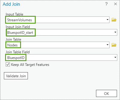
- Verify all tool parameters and click OK.
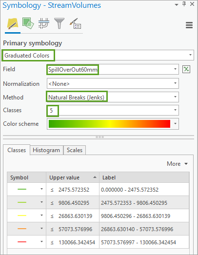
- In the Contents pane, right-click the StreamVolumes layer, then choose Symbology.
- In the Symbology pane, click the Primary symbology drop-down menu and choose Graduated Colors.
- For Field, click the drop-down menu and choose the SpillOverOut60mm field.
- For Method, click the drop-down menu and choose Natural Breaks (Jenks).
- For Classes, choose 5.
- In the Symbology pane, click the Color scheme drop-down menu and choose a color scheme of green to yellow to red.
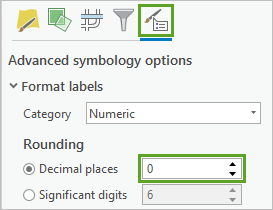
- Click the Advanced Symbology Options, locate Format labels and Rounding. Set the number of Decimal places to 0.
Notice that the class intervals for the StreamVolumes layer are not the same as for the SpillOver60mm layer, although both layers are symbolized using the same SpillOverOut60mm attribute values.
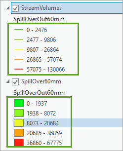
In the StreamVolumes layer, pseudo nodes located where streams merge are included in the join of nodes to streams, so, as streams merge at pseudo nodes, the spillover values increase. However, pseudo nodes located where streams merge are not included in the join of node attributes to bluespots and thus the spillover volumes do not increase.
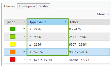
- In the Symbology pane for the SpillOver60mm layer, update the Upper value fields for Classes to be the same class intervals in the StreamVolumes layer.
- For 1937, type 2476.
- For 8072, type 9806.
- For 20684, type 26864.
- For 36859, type 57074.
- Do not change 67775.
Next, exclude streams not carrying any spillover.
- In the Symbology - StreamVolumes pane, click the Advanced symbology options button, then expand Data exclusion.
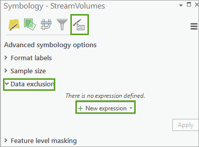
- Click New expression.
- In the Expression builder, add the following expression:
Where SpillOverOut60mm is equal to 0
- Click Apply.
- In the Symbology - StreamVolumes pane, click the Primary symbology button.
- On the Classes tab, locate and double-click the symbol for excluded streams.
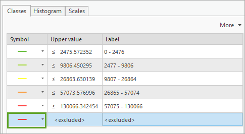
- In the Appearance group, click the red symbol and choose No color.
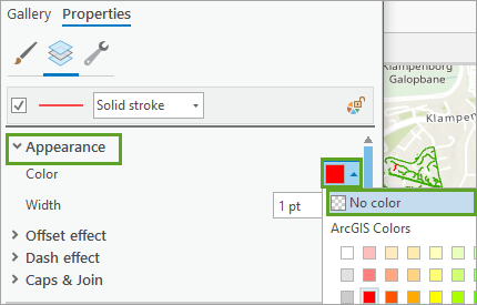
- Click Apply.
The map updates and streams are symbolized based on the spillover volume at the 60 mm event.
- Explore the map and the use bookmarks to investigate specific locations in the study area.
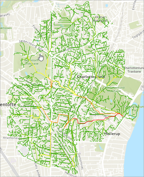
Next, you can illustrate spillovers along the streams by using graduated symbols.
Apply graduated symbology
To apply graduated symbology, complete the following steps:
- In the Investigate Stormwater map, in the Contents pane, right-click the StreamVolumes layer and choose Copy.
- In the Contents pane, right-click Investigate Stormwater and choose Paste.
- Rename the new layer to StreamVolumesBySymbols.
- In the Contents pane, right-click the StreamVolumesBySymbols layer, then choose Symbology.
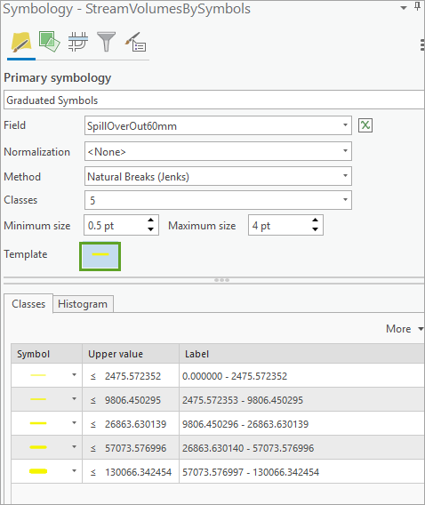
- In the Symbology pane, click the Primary symbology drop-down menu and choose Graduated Symbols.
- For Field, click the drop-down menu and choose the SpillOverOut60mm field.
- For Method, click the drop-down menu and choose Natural Breaks (Jenks).
- For Classes, choose 5.
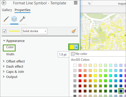
- Click the Template color symbol.
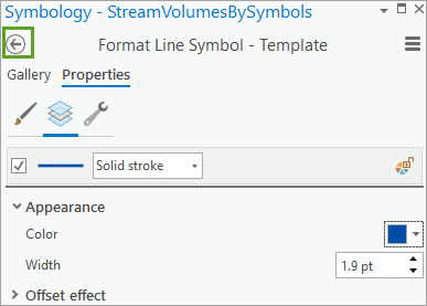
- In the Appearance group, click the Color symbol and choose Blue.
- Click the Return to primary symbology page button.
- In the Symbology pane for the StreamVolumesBySymbols layer, click the Advanced Symbology options button, then expand Data exclusion.
- Click New expression.
- In the Expression builder, add the following expression:
Where SpillOverOut60mm is equal to 0
- Click Apply.
- In the Symbology pane for the StreamVolumesBySymbols layer, click the Primary symbology button.
- On the Classes tab, double-click the symbol for <excluded> streams.
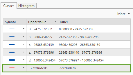
- In the Appearance group, click the symbol and choose No color.
- Click Apply.
- Click the Return to primary symbology page button and review the updated Classes.
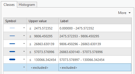
- Explore the map and the use bookmarks to investigate specific locations in the study area.
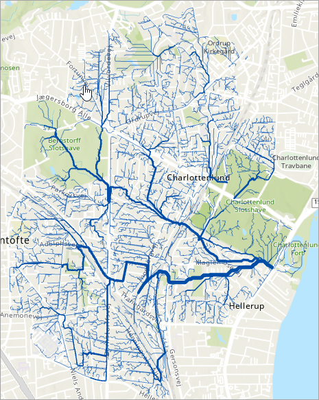
- Save the project.
What did we learn about stream spillovers?
Although this method doesn’t show the actual stream widths, it may provide a better overview of where the biggest water transport corridors are located in the study area. To map the actual widths and depths of the water corridors, kinematic wave equations may be considered, however, this is not currently addressed in the model.
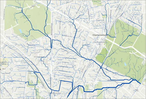
Notice that if a stream’s width abruptly decreases downstream, it is due to a local retention of the runoff in a bluespot having a high capacity, thus reducing the downstream volumes leaving it.
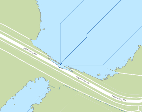
Also, notice how streams in many places are identified along the roads' curbsides, as shown below.
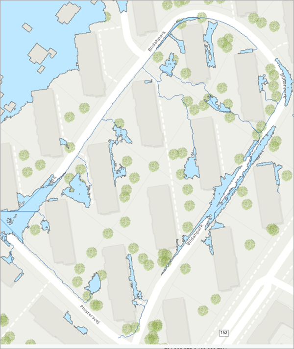
When using a DTM of high precision, a road's centerline is sometimes visible as a drainage divide found along it, forcing the runoff onto the curbsides. That can be verified by swiping the BluespotWatersheds layer on/off when displayed on top of a road map.
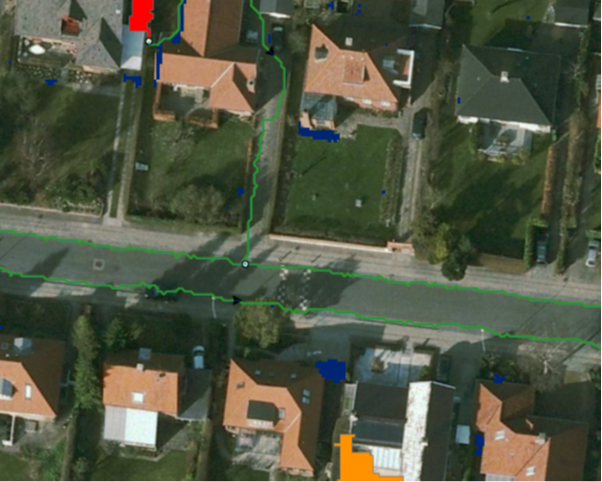
Next, you will map bluespot depths.
Map the bluespots’ depths
The BSDepth layer represents bluespots’ depths in meters, visualized with filled events. In the layer, all minor bluespots not passing the combined depth and volume criteria were omitted. In this section, you will review the bluespot depths.
- In the project, in the original Map, in the Contents pane, select the BSDepth layer, then right-click and choose Copy.
- In the Investigate Stormwater map, in the Contents pane, right-click Investigate Stormwater and choose Paste.

The selected layer is added to the Investigate Stormwater map. Turn off all other layers.
- In the Symbology pane for the BSDepth layer, on the Classes tab, update the Upper values for Classes as follows:
- For 0.40422, type 0.25.
- For 1.126043, type 0.5.
- For 2.367577, type 1.
- For 4.330934, type 2.
- Do not change 7.362587.
- In the Symbology pane, click the Advanced symbology options button.
- For Data exclusion, type 0
The map updates and displays bluespot depths in meters.
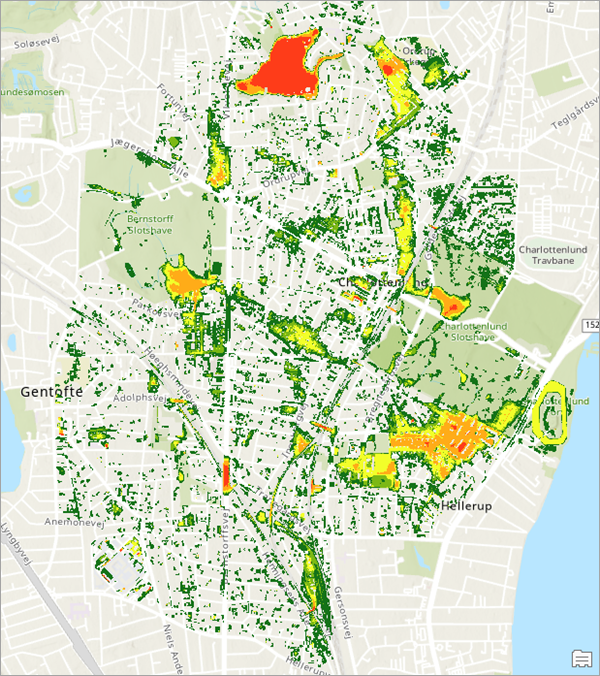
Note:
If all bluespots’ depths need to be considered in your own analysis, use the BSDepthsAll raster located in the project Output.gdb geodatabase. You may use Advanced Symbology Options to apply Data Exclusion and change to manual classification with break values for the first four intervals set at 0.25, 0.5, 1, and 2.
- In the Contents pane, check the BuildingsNoGaps layer and move it above the BSDepths layer. Uncheck all other layers.
- Use bookmarks to explore the map.
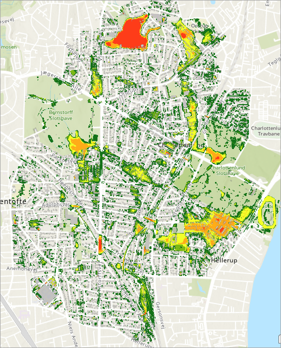
What can we learn about bluespots' depths?
Apparently, several buildings are located critically within the deepest lying parts of the bluespots in the southeastern part of the drainage basin near Hellerup, not far from the basin’s outlet into the sea next to Charlottenlund Fort.
Note that all depths represent bluespots filled to their maximum levels (~ the bluespots’ pour point levels), so bluespot depths should always be compared with the FilledEvent layer.
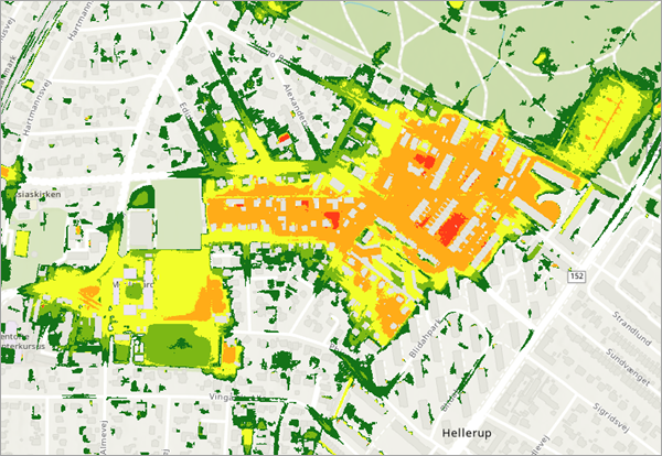
According to the FilledEvent layer, this very large bluespot is filled up at a 70 mm event, and since many buildings are located in the bottom of the bluespot at depths around 2 meters, this area is likely to experience severe flooding problems, even at lower rain events.
Among emergency planners, such a map is popular and named a 'rubber boot index map,' as it tells the teams where to use rubber boots, waders, or sail around in dinghies when rescuing citizens.
Within the study area, classic flooding locations during rainstorms are located at underpasses where roads dip underneath railroad bridges. For an example, review the location at the bookmark named Bernstorffsvej Station.
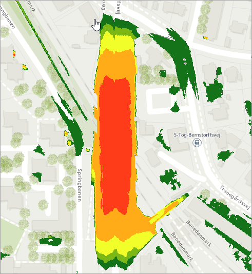
When filled to its pour point level at a filled event of just 30 mm, this bluespot has a maximum depth of a staggering 3.25 meters. Many nonlocal drivers are stuck there during rainstorms when they underestimate its depth.
If you checked the original Streams layer, you will notice that several streams contribute to this major bluespot.
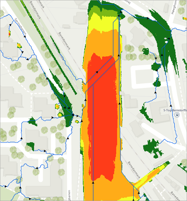
In reviewing the nodes and the pour points in the bluespot’s upper right corner, you will observe that its actual capacity is 15,388 m3, and at a 30 mm event, it produces a spillover of 8,908 m3. When the spillover is this high, it may be dangerous to even walk or drive here because of possible strong currents.
As you can see, the large spillover continues toward the east into a nearby bluespot and then farther eastward until the water moves toward the north along the infrastructure.
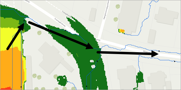
- Continue exploring and when done, save the project.
Challenge - Identify additional locations susceptible to flooding
- During the analysis and exploration of results for the study area, a number of critical locations were identified and discussed. But as a challenge, the author of these lessons would like to encourage you to investigate and try to identify additional locations susceptible to flooding.
- The Inputs.gdb geodatabase associated with the project contains layers with road and rail features. As you have seen, many overpass and underpass locations are particularly susceptible to flooding and at various other local geographic features, overlapping bluespots of various depths may be identified beyond the example already discussed.
- You may also want to consider remediation measures such as how to reduce the downstream spillover by establishing retention or detention basins in existing parks. This can be achieved by studying spillovers at various rain events from bluespots located in upstream parts of the hydrologic network.
- It is possible for you to adjust bluespot storage by manually updating the capacity field from, for example, 1,000 to 10,000 m3 or even more (if feasible) in the Nodes layer and re-executing the SpillOver_Batch tool. In this way, it would be possible to detect a decrease in downstream spillovers and the reduction in the number of affected buildings at specific rain events.
- During your exploration, you may realize how the bluespot modeling tools might be efficient in the planning of detention basins near future site developments and where to avoid new constructions.
- For now, you have completed an exploration of the Charlottenlund study area.
In the next module, you will focus on how to prepare data from your own study area for the bluespot modeling.
Run the analysis with your own data
You can think of this module as a road map to investigating data requirements, data preparation steps, and associated tools used to create bluespots for predicting flood risk assessment due to storm water incidents in your own study area. Steps and suggestions in this module will assist you in using the associated modeling tools to screen a digital terrain model for landscape depressions within a drainage basin, locate their hierarchical downstream locations, and predict how they will be filled up and spill over during simulated uniform rainstorms.
In preparation for performing your own bluespot analysis on local data for your study area, you need to be aware of several data considerations and preparation steps as outlined next.
For the modeling process, you will need a terrain model constructed from ground points on bare earth. If building footprints are available, these may be incorporated to improve the modeling results.

For an overview of the hydrologic modeling tools in the ArcGIS Spatial Analyst extension, it is recommend that you review the Hydrologic analysis sample applications topic.
Prepare your own data - elevation model considerations
In bluespot modeling, a strong recommendation is to aim at using a digital terrain model (DTM) constructed from ground points on bare earth (and optionally with building elevations added), and not a digital surface model (DSM) that includes combinations of vegetation heights and buildings.
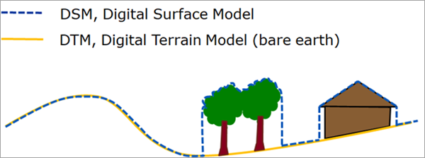
See Exploring digital elevation models for more information.
During modeling, it is noticeable that when using a DSM, many false bluespots are discovered in between tree canopies or in between tree canopies and buildings. When detected, huge nonexistent bluespot volumes and false runoff flow paths may be created.
Unfortunately, a high-resolution DTM is far more expensive to produce than a DSM, so very few are publicly available as open geospatial data. As a result, you may consider using a DTM of lower resolution, for example, 10 or 30 meters if available. Although imprecise and coarse-grained and possibly not free from artifacts, it may still provide interesting overviews.
Note:
Some countries, such as Denmark, openly share lidar-based national elevation models with spatial resolutions of 0.4 meters. For more information, visit the Danish Agency for Data Supply and Efficiency website. For data, you may visit the following download site and select data for use in this lesson.
Another way of obtaining a DTM is to build it yourself from datasets created by a UAV-mounted lidar sensor system. With the processed DTM, it should be straightforward to use it in bluespot modeling. Keep in mind that the DTM should cover an entire drainage basin—or at least a subset that doesn't have any upstream contributions.
Hydrologic conditioning refers to the modification of topographic data in a raw or “bare earth” digital elevation model (DEM) through a series of GIS processing steps to more accurately represent the movement of water across the landscape.
It is important to note that the most trustworthy storm water scenarios are produced from using a hydro-conditioned DTM with buildings added to divert runoff around them. See An overview of the Hydrology toolset for more information on tools that may be used for this purpose.
Note that this lesson does not provide a workflow to upgrade your DTM to a hydro-conditioned version (DHyM). However, the associated project contains a BluespotScreeningSupplements toolbox, with a tool named Burn Buildings Onto DTM, which provides a method to add building footprints to your DTM.
Note:
For more information on hydro-conditioning, it is recommended that you explore the ArcHydro extension for ArcGIS Pro to learn more about how you may produce a hydro-conditioned DTM yourself. In addition, you may review the following resources:
In the next section, you will create and set up a project to perform your own bluespot analysis.
Data preparation - set up your bluespot project
ArcGIS Pro organizes all necessary data, maps, and tools in a project folder, keeping all required components together and thereby facilitating management and sharing. In this section, you will learn to apply the workflow to your own data.
- On the ribbon, in the Map tab, in the Layer group, click Add Data.
- In the Add Data window, navigate to a location of your choice and on the ribbon, click New Item and select Folder.
- Rename the folder MyStudyArea or a name of your choice.
- Click the Project tab, then click Options.
In the Change settings for the current project pane, review the current Home folder, Default geodatabase, and Default toolbox settings for the project.
- Verify the Home folder setting and, if necessary, update the location to your project folder location.
- Verify the Default geodatabase setting and, if necessary, update the location to your project’s output geodatabase.
The Outputs geodatabase stores output data generated by the modeling tools.
- Verify the Default toolbox setting, update the toolbox to the BluespotScreening.tbx file in your project folder.
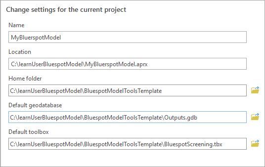
Note:
Before continuing, ensure that all your data (the elevation model and optional building footprints) is projected and that the planar unit and the elevation data's z-unit are in meters. If not, all area and volume calculations produced by the model tools will be inaccurate.
To verify the data units, in the Catalog pane, right-click the data source and select Properties -> General -> Spatial Reference. Then identify the projected coordinate system’s linear unit. This must be meters; if not, use the project tool update the data source to a projection with linear units in meters.
- Save the project.
- In the Catalog pane, expand Inputs.gdb and add your project feature classes.
You may copy or import the feature classes into the Inputs geodatabase, or add a folder connection to an existing geodatabase containing your input data and DTM. Copying a feature class may only be done between geodatabases; if your data is in a non-geodatabase format, you would need to import instead of copying.
Note:
Review the Feature Class To Feature Class conversion tool for how to import data into a geodatabase.
Your model data may include the following:
- DTM
- Building footprints
- Roads
- Railroads
These feature classes represent your processed data to be used in the tools and model to predict the flooding consequences from storm water events.
- In the Catalog pane, expand the BluespotScreening toolbox and review the collection of bluespot modeling tools and scripts. Note the Identify Bluespots Features model.
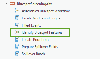
- In the Catalog pane, expand the BluespotScreeningSupplements toolbox and review the data preparation tools and scripts available to update and modify your input datasets to identify bluespot features.
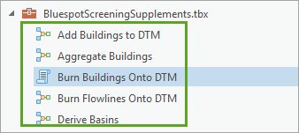
- Save the project.
Next, you will review the data preparation steps and tools available to process your input data.
Data preparation - derive a drainage basin
Now that you have set up your project and have collected and added input data to the necessary geodatabase, you need to initiate several data housekeeping steps to make the modeling efficient and useful.
The first consideration is to ensure you include the extent of the entire drainage basin affecting your area of interest. In other words, it does not make sense to execute the model on the area of a city where the extent of the city does not include the entire drainage basin in which it is located. Accurate hydrologic modeling depends on the location of the major drainage divide a study area falls within.
To derive the drainage basin for your study area, prepare the DTM by filling all sinks at their pour points, then use the Basin tool available in the ArcGIS Spatial Analyst extension.
The following example illustrates the drainage basins derived from a DTM covering the Charlottenlund case area. The outcome shows several minor drainage basins presented in different colors around the Charlottenlund drainage basin presented in yellow.
Note:
There is no reason to include additional drainage basins (or parts thereof) in the screening ahead than the basin or basins covering the area of interest, as the neighboring basins don't affect the area of interest's surface hydrology.
The following is the workflow you may follow to generate and extract the basin relevant to your study area.
- In the Catalog pane, expand the BluespotScreeningSupplements toolbox, right-click the Derive Basins model, then choose Edit.
Review the model steps; when done, close and do not save changes.
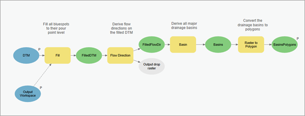
- In the Catalog pane, in the BluespotScreeningSupplements toolbox, double-click the Derive Basins model tool.
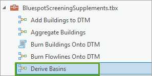
- In the Derive Basins tool, for DTM, choose your project DTM and ensure your Output Workspace is set correctly.
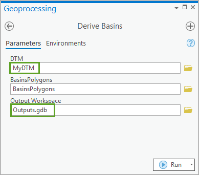
- Click Run.
The model executes, and a layer named BasinPolygons is added to the Bluespot Model Map.
- Use the Select tool to select the polygon representing your project area drainage basin from BasinPolygons.
- Use the Extract by Mask tool (Spatial Analyst) to cut out the selected basin data from your input DTM.
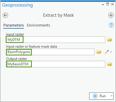
After extracting the DTM for the basin applicable to your study area, you are ready to execute the Identify bluespot features model. However, you should consider incorporating buildings into your DTM to enable flows around structures and to eliminate the buildings' volumes if they are located within a bluespot. If you choose not to incorporate structures, you may continue by executing the model.
Data preparation - add buildings to DTM (optional)
If you can provide a feature class of building footprints for your study area, it would greatly enhance the results of the model if you were able to 'stamp' them onto the DTM. However, you do need to prepare the building layer by eliminating tiny slivers in between adjacent buildings having widths lesser than or equal to the cell size for the DTM used, and you need to identify and fill gaps inside closed building complexes such as courtyards.
The illustration below shows a small subset of building features. The left shows the before situation with a small sliver between adjacent buildings and gaps inside closed building complexes. The right shows the same buildings after execution of the Add Buildings to DTM model and illustrates how courtyards 1 and 2 were filled, but that courtyard 3 was not filled, as the gap between buildings did not meet the sliver elimination criteria (slivers between adjacent buildings must have a width less than or equal to the cell size of the DTM used).
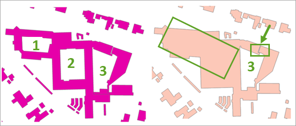
How the Add Buildings to DTM model works
The Add Buildings to DTM model first calls and executes the Aggregate Buildings model to eliminate the tiny slivers in between adjacent buildings and identify and fill gaps inside closed building complexes (courtyards) using the Union tool. Finally, it passes the results to a script named Burn Buildings Onto DTM that burns the BuildingsUnioned features onto the DTM.
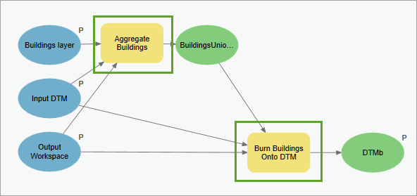
During its execution, all building polygons are converted to a temporary raster dataset with the same cell size as the DTM. During the conversion, an elevation value of 30,000 is assigned to the building raster’s cells and stamped onto the DTM. Later, when modeling storm water flows, the closed buildings force the surface runoff around them, and the precipitation falling on the ‘closed rooftops’ floats down along the buildings' sides (although the exact flow directions over the rooftops cannot be controlled).
If you have building polygons, follow these steps to execute the Add Buildings to DTM model:
- In the Catalog pane, in the BluespotScreeningSupplements toolbox, double-click the Add Buildings to DTM model tool.
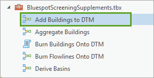
- In the Add Buildings to DTM tool, for Input DTM, choose the DTM covering the basin for your study area. Next, provide your building layer and ensure your output workspace is set correctly, then click Run.
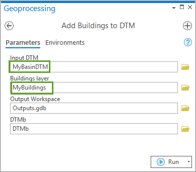
The Add Buildings to DTM model executes and the resulting DTM now incorporates building footprints that have slivers between adjacent buildings eliminated and gaps inside closed building complexes filled.
The illustration below shows the incorporation of structures into the Charlottenlund drainage basin DTM.
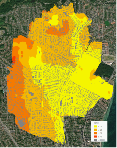
Data preparation - burn flow lines onto the DTM
When using DTMs to model water flow, it is strongly advised that the DTM be hydro-conditioned before modeling. However, hydro-conditioning is not a single step but rather a multistep process necessary to incorporate topographic features that determine flow paths that may not be captured in a source DTM.
Note:
If you have not reviewed details on hydro-conditioning, consult the following slide presentation for a detailed description of a hydro-conditioning workflow.
An important component of bluespot modeling is the role played by flow paths along roads passing under other roads (for example, roads not intersecting but crossing at different elevations, such as freeways). Additional consideration needs to be given to flow paths along streams and channels passing under roads, streams passing under bridges, and flows along road and railroad tunnels.
Advanced hydro-conditioning tools are available in ArcGIS and it is strongly recommended that you apply and use these on your DTM. However, a simple model named Burn Flowlines Onto DTM is provided with the bluespot modeling tools to help you adjust flow paths and incorporate quick hydro-conditioning approximation into your DTM.
An example of where the Burn Flowlines Onto DTM model will make a difference is illustrated below.
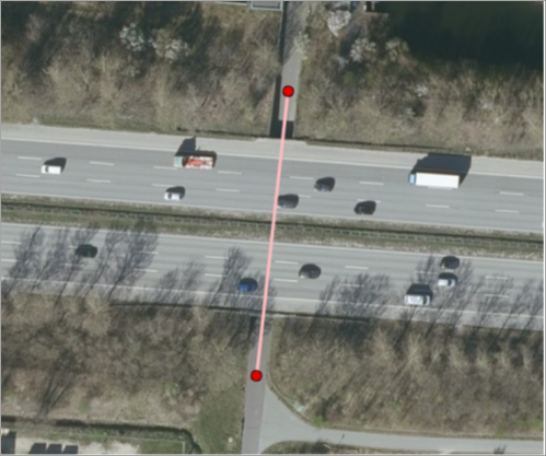
The illustration shows a situation where a cycle track follows a path under a freeway. The cycle track is not incorporated into the original DTM and thus no flow path is identified.
What the Burn Flowlines Onto DTM model does is incorporate cut flow lines (hydro adaptions) into the DTM, enabling water to flow along them. The illustration below shows the incorporation of the cycle track that passes under the freeway incorporated into the DTM.
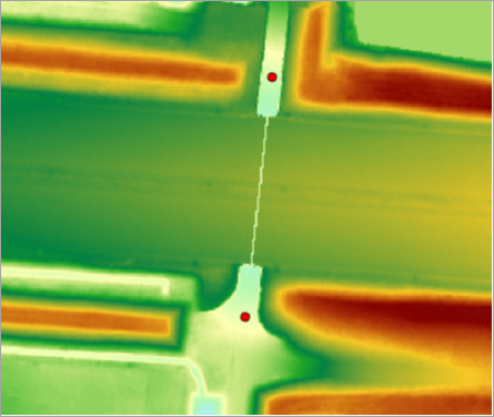
Note:
To incorporate flow lines, you need to generate hydro adaptions (line features) by digitizing and providing them for inclusion into the DTM. The hydro adaptions must be digitized manually from high-resolution orthophotos completely matching the DTM to be adjusted.
- In the Catalog pane, in the BluespotScreeningSupplements toolbox, double-click the Burn Flowlines Onto DTM model tool.
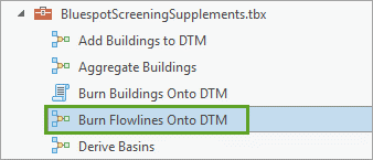
- In the Burn Flowlines Onto DTM model tool, for Input Hydro Adaptions, provide the line feature layer. For Input DTM, provide the DTM covering the basin for your study area. Ensure your output workspace is set correctly, then click Run.
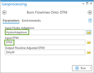
How the Burn Flowlines Onto DTM model works
For all line features, the model locates the lines' endpoints, and assigns elevation values to them extracted from the DTM.
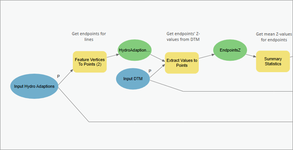
For each line feature, the two endpoints' z-values are averaged, joined onto the line feature attribute table, and used as the value to be assigned to the cells during a line to raster conversion. The output is a temporary raster that is stamped onto the DTM.
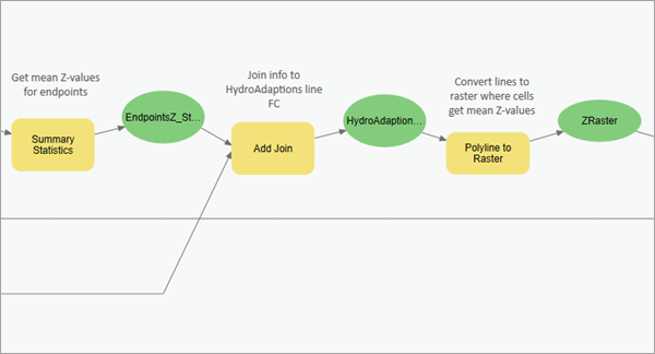
When done, water flows are enabled at the approximated z-level through one cell wide hydrologic flow paths.
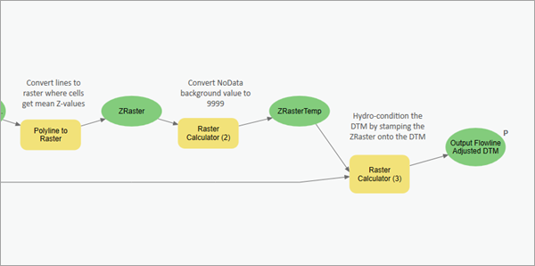
Note:
Flow paths generated by the Burn Flowlines Onto DTM model are not hydraulically correct, but hydrologically correct only.
Congratulations, you have now completed data preparation for your study area and are ready to perform bluespot modeling on your source data.
Execute the Assembled Bluespot Workflow model
The Assembled Bluespot Workflow model, located in the BluespotScreening toolbox, is available for you to execute all five bluespot modeling steps in a single process.

You may want to review the model before setting parameters and running the processes.
For a detailed exploration of all model steps, consult the Run the model and tools module.
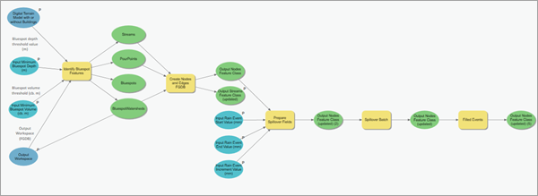
In the first part of the model, you specify the input DTM (optionally including buildings), threshold values for the bluespots' minimum depth (m) and volume (m3), and the Output Workspace location. These input parameters are passed to the Identify Bluespot Features model.
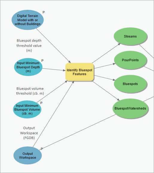
Outputs from the Identify Bluespot Features model are passed to the Create Nodes and Edges FGDB script, which prepares the hydrologic network to trace the accumulated downstream spillover from the bluespots pour points along the detected flow paths, representing your derived streams.
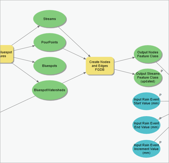
Next, nodes and the updated streams are passed to the Prepare Spillover Fields script, which prepares nodes and passes them to the Spillover Batch script to calculate the downstream accumulated spillover from one bluespot to the next bluespot or bluespots downstream.
And lastly, the Filled events script calculates the downstream accumulated spillover, allowing you to look up the smallest rain event producing a spillover from a bluespot in the Nodes attribute table.
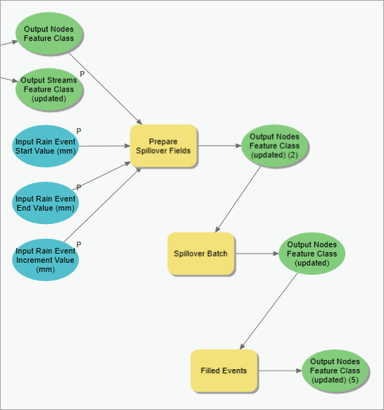
When you are ready to execute the Assembled Bluespot Workflow model located in the BluespotScreening toolbox, double-click the model.
The tool parameters include the following:
- Digital Terrain Model with or without Building
- Bluespot volume threshold (cm3)
- Bluespot depth threshold value (m)
- Output Workspace
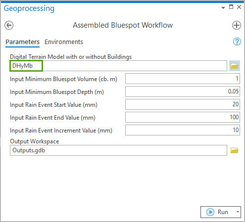
In this set of modules, you learned how to perform a storm water impact assessment for a drainage basin in Denmark. The modeling was based on a screening for local landscape sinks (bluespots), their capacities and locations in a hydrologic network, and when spilling over, you detected the overall flow paths.
After the modeling, you were able to predict areas of high and lower risk of getting flooded in storm water situations. As the modeling was carried out in a timeless environment and assuming 100 percent runoff of the precipitation falling on the terrain, the results should be considered as first approximations of impacts only. However, valuable information can be obtained about areas more vulnerable to storm water incidents than other, and where new site developments should be carefully considered apart from water corridors and sinks.
Meanwhile, many considerations about potential locations of new retention and detention basins, redirection of flow paths, and local establishment of protective dikes can be discussed before taking the investigations to higher levels in collaboration with advisors from consultancy companies and involving more professional software.
References
Below is a list of references demonstrating some potentials of the bluespot screening method.
- Balstrøm T & Crawford D (2018): Arc-Malstrøm: A 1D hydrologic screening method for stormwater assessments based on geometric networks. Computers & Geosciences. 116, p. 64-73. DOI: Arc-Malstrøm: A 1D hydrologic screening method for stormwater assessments based on geometric networks
- Mhina GJ, Jensen BM, Mbuligwe SE, Kassenga GK & Balstrøm T (2021):GIS-based flood proneness screening: A prelude to stormwater management in fast urbanizing catchments. Frontiers of Earth Science. In press.
- Thrysøe C, Balstrøm T, Borup M, Jamali B & Arnbjerg-Nielsen K (2021): FloodStroem- A fast dynamic GIS-based urban flood and damage model. J. of Hydrology, 2021-09. DOI: FloodStroem: A fast dynamic GIS-based urban flood and damage model
- Trepekli K, Balstrøm T, Friborg T, Fog B, Allotey AN, Kofie R & Møller-Jensen L: UAV-LIDAR observations increase the precision of urban flood modelling in Accra by detecting critical micro-topographic features. Submitted to Natural Hazards.
- Westergaard-Nielsen A, Balstrøm T, Treier U, Normand S & Elberling B (2020): Estimating meltwater retention and associated nitrate redistribution during snowmelt in an Arctic tundra landscape. In: Environmental Research Letters. 15, 3, 13 p. DOI: Estimating meltwater retention and associated nitrate redistribution during snowmelt in an Arctic tundra landscape
- Zhao G, Balstrøm T, Mark O, Jensen MB (2021): Multi-scale target-specified sub-model approach for fast large-scale high-resolution 2d urban flood modelling. Water, 2021, 13(3), 259. DOI: Multi-Scale Target-Specified Sub-Model Approach for Fast Large-Scale High-Resolution 2D Urban Flood Modelling

