Create a NetCDF file

You'll use the Ecological Marine Units (EMU) feature class of the Caribbean Sea to create a NetCDF file using Python using ArcGIS Pro. First, you'll set up a new project from a project package. Second, you'll start a new Python Notebooks. Third, you'll create an empty NetCDF file with the EMU schema. Lastly, you'll load the EMU values into the NetCDF file. The output EMU NetCDF file will have the required format to be loaded and visualized as a voxel layer in ArcGIS Pro.

Set up a new project

You'll start a new ArcGIS Pro project using a project package. This package contains the country and a sample of EMU data. First, you'll process this EMU data using an ArcGIS Notebooks.

Download the project package and double-click it to open it in ArcGIS Pro. If prompted, sign in to your ArcGIS account.
Note:
If you don't have access to ArcGIS Pro or an ArcGIS organizational account, see options for software access.
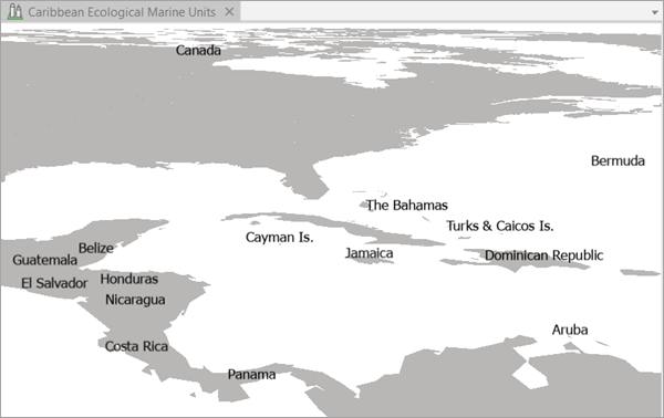
The project contains the Caribbean Ecological Marine Units local scene and the EMU_Caribbean_Sea 3D points feature class.
Note:
You can turn on the World Ocean Base layer and the WorldElevation3D/TopoBathy3D layer (and turn off the Countries layer) for better geographic reference. The less data on the map, the faster it will draw.
On the ribbon, click the Insert tab and choose New Notebook.

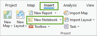
A new notebook is added to the project. Notebooks details can be edited in the Catalog pane.
In the Catalog pane, expand the Notebooks folder.
Right-click New Notebook.ipynb and choose Rename.
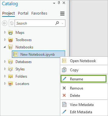
Type Create EMU NetCDF file.ipynb and press Enter.
A new ArcGIS Pro project with a local scene and an empty Python notebook are ready.

Create an empty NetCDF file

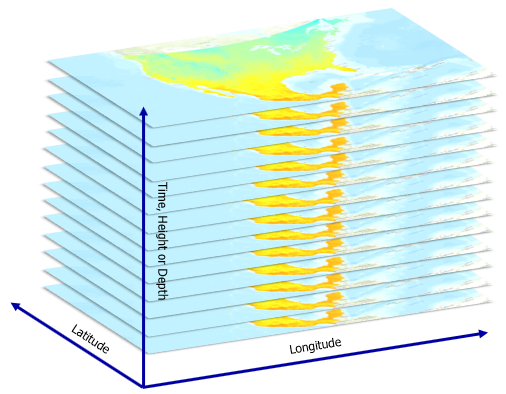
First, you'll create a NetCDF file for the EMU in the Caribbean Sea. The NetCDF file will be built in a latitude, longitude, and depth grid. The file will also include global attributes, dimensions, and variables. These are the foundational attributes needed to map (latitude, longitude, and depth) and display the associated variables (temperature, salinity, and oxygen) in 3D.

Multidimensional data collected over space and time, depth or height

In the notebook's empty cell, type the following commands to load the required Python modules:
```
import os
import arcpy
import netCDF4
import numpy as np
import datetime as dt
```
These modules are the libraries that contain the functions used in the script. For example, the arcpy module has the ArcGIS geoprocessing, data management, and mapping functions. The netCDF4 module allows us to read and write NetCDF files.
On the Notebooks ribbon, click Run.

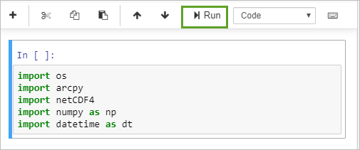
Once the first cell runs, the braces will show the number 1. A new cell is added below the first.
Note:
You can add new cells from the notebook ribbon by clicking the Insert tab and choosing Insert Cell Below.
In the new cell, paste the following commands related to the output NetCDF file and the regular 3D grid and click Run:
```
# Output file
output_nc = "EMU_Caribbean_Voxel.nc"

# Grid
lowerleft_x = -88.625
lowerleft_y = 8.375
cellsize = 0.25

# Number of cells
no_rows = 58
no_cols = 117
no_depths = 101

# Values
lat_vals = np.arange(lowerleft_y, lowerleft_y + cellsize*no_rows, cellsize)
lon_vals = np.arange(lowerleft_x, lowerleft_x + cellsize*no_cols, cellsize)
z_vals = np.arange(0, -505, -5)

# Print vectors
print('Latitude')
print(lat_vals)
print('Longitude')
print(lon_vals)
print('Depth')
print(z_vals)
```
Each variable definition is broken up with associated comment (#). Output_nc specifies the name of the output NetCDF file. Lowerleft_x and lowerleft_y specify the coordinates for the NetCDF file. Cell size represents the resolution of 1/4 degree. No_rows specifies the number of rows, which is affiliated with latitude; in this case, 58 rows at 0.25 cell size means 14.5 degrees of latitude. No_cols specifies the number of columns, which is affiliated with longitude; in this case, 117 columns at 0.25 cell size means 29.25 degrees of longitude. This means that the output will be a little more than twice as wide (longitude) as it is long (latitude). No_depths specifies the number of depth values that will be included in the NetCDF file. This represents our water column space in 3D. In the next variable definition (Values), you specify how these can all be used together to produce a regularly spaced horizontal grid and irregularly spaced vertical (depth) grid.
The latitude, longitude, and depth vectors are printed on the screen.
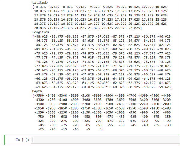
Next, you will create an empty NetCDF file using the Dataset function of the netCDF4 Python module. You will also provide global attributes to add documentation to the file.

In the empty cell, paste the following code and click Run:

# Create File
nc_file = netCDF4.Dataset(output_nc, 'w', format="NETCDF4", set_auto_mask=False)

# Global Attributes
nc_file.title = 'Ecological Marine Units'
nc_file.summary = 'Ecological Marine Units (EMUs) for the Caribbean Sea.'
nc_file.keywords = 'Global, EMU, USGS, NOAA, Esri, 3D, Ocean, Marine, Ecology'
nc_file.license = ('This work is licensed under a Creative Commons Attribution 4.0 '
                   'International License.')
nc_file.references = ('Please see references Cited in this publication: ' 
                    'http://www.aag.org/galleries/default-file/AAG_Marine_Ecosyst_bklt72.pdf')
nc_file.source = 'Esri, USGS,  NatureServe, GEO, NOAA, NASA, NIWA'
nc_file.Conventions = 'CF-1.6'
nc_file.institution = 'Esri'
nc_file.history = ('{0} Creation of EMU Caribbean '
                   'netcdf file.').format(dt.datetime.now().strftime("%Y-%m-%d"))

Note:

It is fundamental to document a NetCDF file so other people can understand it better. You can follow the Climate and Forecast (CF) Metadata Conventions to guide you on standard attributes and variable names.

In a new cell, copy and paste the following code to create the latitude, longitude, and depth dimensions:
```
# Create Dimensions
lat_dim = nc_file.createDimension('latitude', no_rows)
lon_dim = nc_file.createDimension('longitude', no_cols)
top_dim = nc_file.createDimension('depth', no_depths)
```
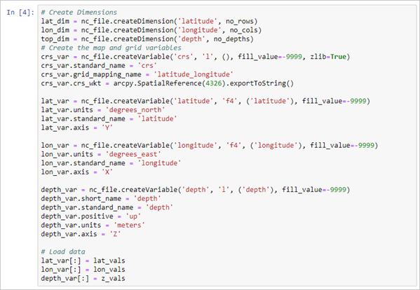
Next, you will add code for mapping and gridding variables: crs, latitude, longitude, and depth and load the lat_vals, lon_vals, and z_vals vectors into their respective (in other words, lat_var, lon_var, and depth_var) variables.

At the end of the same cell, add the following code and click Run:

# Create the map and grid variables
crs_var = nc_file.createVariable('crs', 'l', (), fill_value=-9999, zlib=True)
crs_var.standard_name = 'crs'
crs_var.grid_mapping_name = 'latitude_longitude'
crs_var.crs_wkt = arcpy.SpatialReference(4326).exportToString()

lat_var = nc_file.createVariable('latitude', 'f4', ('latitude'), fill_value=-9999)
lat_var.units = 'degrees_north'
lat_var.standard_name = 'latitude'
lat_var.axis = 'Y'

lon_var = nc_file.createVariable('longitude', 'f4', ('longitude'), fill_value=-9999)
lon_var.units = 'degrees_east'
lon_var.standard_name = 'longitude'
lon_var.axis = 'X'

depth_var = nc_file.createVariable('depth', 'l', ('depth'), fill_value=-9999)
depth_var.short_name = 'depth'
depth_var.standard_name = 'depth'
depth_var.positive = 'up'
depth_var.units = 'meters'
depth_var.axis = 'Z'

# Load data
lat_var[:] = lat_vals
lon_var[:] = lon_vals
depth_var[:] = z_vals

The crs variable does not have any dimensions or variables; it provides the mapping spatial reference information.

Codeblock to create the output file and load data

In a new cell, paste three variables for the EMU data: sea water temperature, salinity, dissolved oxygen, and cluster37, and click Run.

# Create EMU Variables
temp_var = nc_file.createVariable('temp', 'f4',
                                  ('depth', 'latitude', 'longitude'), fill_value=-9999)
temp_var.short_name = 'temp'
temp_var.standard_name = 'sea_water_temperature'
temp_var.units = 'degree_Celsius'
temp_var.grid_mapping = 'crs'

sali_var = nc_file.createVariable('salinity', 'f4',
                                  ('depth', 'latitude', 'longitude'), fill_value=-9999)
sali_var.short_name = 'salinity'
sali_var.long_name = 'sea_water_salinity'
sali_var.units = ''
sali_var.grid_mapping = 'crs'

dissO2_var = nc_file.createVariable('dissO2', 'f4',
                                  ('depth', 'latitude', 'longitude'), fill_value=-9999)
dissO2_var.short_name = 'dissO2'
dissO2_var.long_name = 'mole_concentration_of_dissolved_molecular_oxygen_in_sea_water'
dissO2_var.units = 'microliters/liter'
dissO2_var.grid_mapping = 'crs'

cluster37_var = nc_file.createVariable('cluster37', 'l',
                                       ('depth', 'latitude', 'longitude'), fill_value=-9999)
cluster37_var.short_name = 'cluster37'
cluster37_var.long_name = 'cluster37_id'
cluster37_var.units = ''
cluster37_var.grid_mapping = 'crs'

Sea water temperature, salinity, and dissolved oxygen are key variables used for the characterization of the ocean and its environmental condition. The cluster variable holds the classification of a grid cell within the EMU dataset. Notice that the first three variables have a floating number data type (in other words, ‘f4') while the cluster37 variable has an integer number data type (in other words, ‘l').

Note:

For this tutorial, a subset of data for the Caribbean sea for a depth of 500 meters was used. Visit the Ecological Marine Units (EMU) web app in ArcGIS Living Atlas of the World to learn more about the EMU dataset. The complete EMU dataset contains more variables than the three listed in this exercise. You can download the full EMU NetCDF file from ArcGIS Online.

Load data into the NetCDF file

Next, you'll load the values from the EMU point feature class into the NetCDF file.

In the Contents pane, right-click the EMU_Caribbean_Sea feature class and choose Attribute Table.

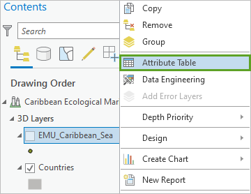
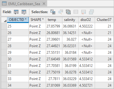
The attribute table appears.
The temp, salinity, dissO2, and Cluster37 fields for each 3D point (coordinates X, Y, and Z) contain the information that will be loaded into the NetCDF file variables.
Close the attribute table.
In a new cell at the end of the notebook, assign the EMU_Caribbean_Sea feature class into the fc variable. Create a Search Cursor with the fc variable and the fields: temp, salinity, dissO2, Cluster37, and Shape@. Do not run the cell yet.
```
# Load EMU data
fc = os.path.abspath(r'.\EMU.gdb\EMU_Caribbean_Sea')
cursor = arcpy.da.SearchCursor(fc, ['temp', 'salinity', 'dissO2', 'Cluster37', 'Shape@'])
```
In the Contents pane, double-click the EMU_Caribbean_Sea layer. In the Layer Properties window, click the Source tab.
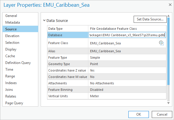
Copy the source path from the Database row and paste it into the notebook as the fc path variable. Make sure to include the file name EMU_Caribbean_Sea at the end.

In the same cell, use a for loop to iterate over the rows in the cursor. Get the EMU variable values, replace null values with -9999, get the array indices for the 3D point, and store the variable values in the NetCDF array.

# For each record in the table
for row in cursor:
    # Get values
    temp, salinity, dissO2, cluster37 = row[:4]
    coords = row[4].getPart()
    # Replace null values with -9999
    temp = float(temp) if temp else -9999
    salinity = float(salinity) if salinity else -9999
    dissO2 = float(dissO2) if dissO2 else -9999
    cluster37 = float(cluster37) if cluster37 else -9999
    # Get indices in array of current 3D point
    idx = (np.abs(lon_vals - coords.X)).argmin()
    idy = (np.abs(lat_vals - coords.Y)).argmin()
    idz = np.where(z_vals==int(coords.Z))[0]
    # Store variables values
    if idz.size > 0:
        temp_var[idz, idy, idx] = temp
        sali_var[idz, idy, idx] = salinity
        dissO2_var[idz, idy, idx] = dissO2
        cluster37_var[idz, idy, idx] = cluster37
del(cursor)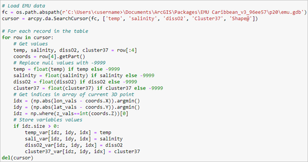

For loop that will iterate over the rows in the cursor

Run the cell.
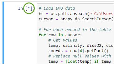
The cell may take some time to run. When a cell is running, an asterisk (*) appears next to the cell. It will become a number when it is complete.
In a new cell, copy and paste the following code to close the NetCDF file and click Run.
```
# Close NetCDF file
nc_file.close()
```
Tip:
You can download the final Python notebook from ArcGIS Online.
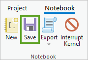
On the ribbon, on the Notebook tab, click Save.

You've created an empty NetCDF file. You also loaded values into the NetCDF file from a point feature class using Python Notebooks in ArcGIS Pro. Next, you'll load this NetCDF file as a multidimensional voxel layer in a local scene.

Add a NetCDF file as a voxel layer

Previously, you created a NetCDF file using Python notebooks in ArcGIS Pro and the EMU point feature class. Next, you'll load the EMU NetCDF file in a local scene as a multidimensional voxel layer. The voxel layer can be used to visualize EMU variables such as sea water temperature, salinity, or dissolved oxygen in 3D.

Add a multidimensional voxel layer

First, you'll add the EMU NetCDF file as a voxel layer.

Click the Caribbean Ecological Marine Units tab to open the local scene.
On the ribbon, on the Map tab, click the Add Data drop-down arrow and choose Multidimensional Voxel Layer.
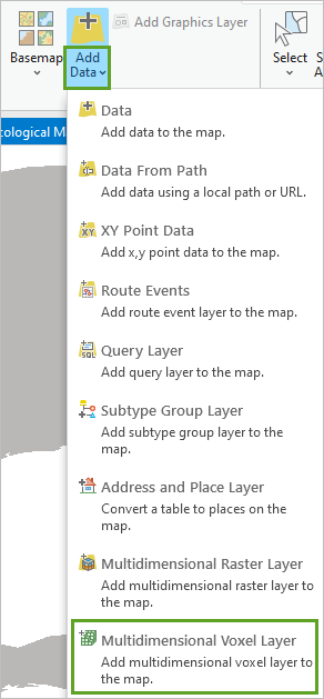
The Add Voxel Layer window appears.
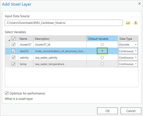
In the Add Voxel Layer window, for Input Source Data, click Browse and choose the EMU_Caribbean_Voxel.nc file.
Once you choose the file, the available attribute fields will populate the Select Variables section.
Each variable defined in the NetCDF file is listed in the Add Voxel Layer window. You can decide which variables to include in the voxel layer by checking the variables on or off. You can choose which variable to set as the default variable. When the voxel layer gets added to the scene, this will be the variable shown.
A variable has a defined data type that determines how the variable can be symbolized. For example, a continuous data type could be numeric values such as sea water temperature, salinity, or dissolved oxygen. The continuous variables can be visualized using stretch values. In cases in which the data type is discrete like cluster37, you can symbolize the variable using unique values.
For Select Variables, in the Default Variable column, set dissO2 as the default.
Click OK.

The EMU NetCDF file appears as a voxel layer in ArcGIS Pro.
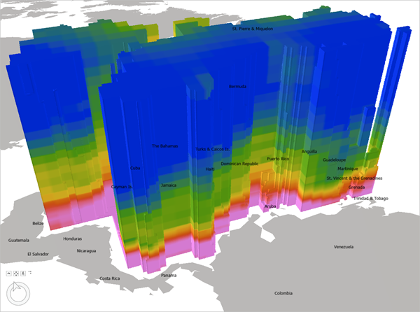
It's currently drawn with default colors and elevation values. To more accurately visualize this data, you'll change the elevation and styling.

This layer is currently drawing on top of the ocean. To correctly place it at depth, you'll set the vertical exaggeration.
In the Contents pane, click the EMU_Caribbean_Voxel layer to select it.
On the ribbon, click the Voxel Layer tab.
In the Elevation group, for Vertical Exaggeration, delete the negative sign so it is set to 3223.86.
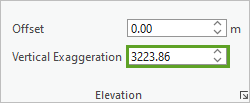
The voxel layer updates in the scene.

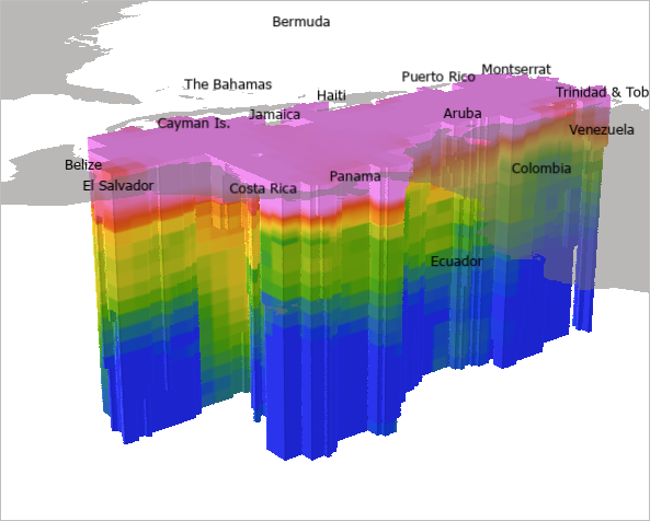
Next, for visualization purposes, you'll apply a style developed specifically for showing oceanographic data. The oceanographic style includes a variety of color schemes designed to visualize characteristics such as oxygen level in the ocean. The color range and label need to match to make it easy for your audience to interpret the values in the voxel layer.
Download the cmocean.stylx style package.
On the ribbon, click the Insert tab. In the Styles group, click Add and choose Add Style.
In the Add a style file window, choose the cmocean.stylx file and click OK.
Note:
If the Upgrade Style window appears, click Yes to continue.
Now you can apply the style to the layer.
On the ribbon, click the Voxel Layer tab. In the Drawing group, click Symbology.
The Symbology pane appears.
In the Symbology pane, for Color Scheme, expand the menu and check Show names and Show all.
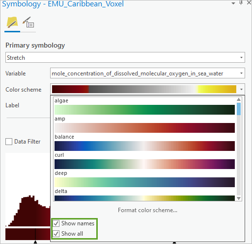
The ocean styles you downloaded are shown at the top of the list.
Find and select the oxy color scheme.
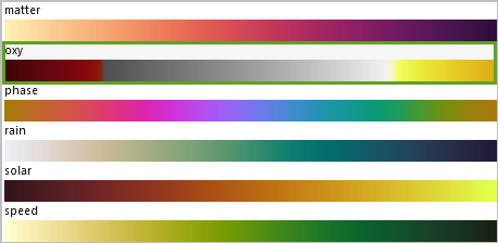
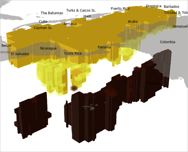
The map redraws to show the new color scheme. A low concentration of dissolved oxygen is shown in reds and maroons, while a high concentration is shown in yellows.

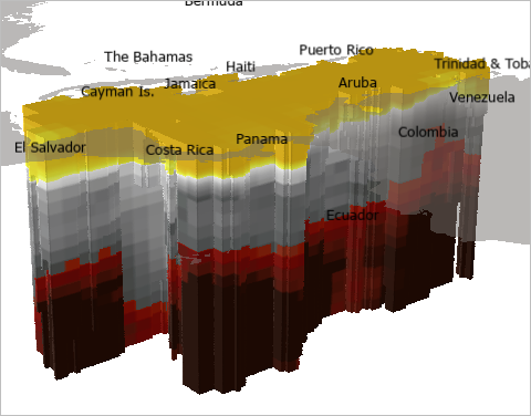
The middle values are shown in gray. To emphasize high and low values, you'll use transparency to hide these intermediate values.
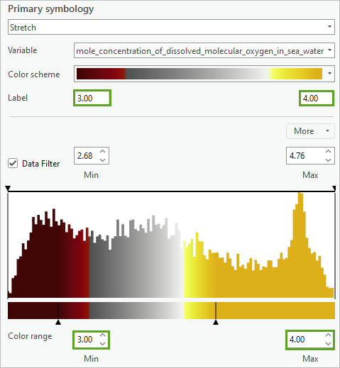
In the Symbology pane, for Label and Color range, set the Minimum value to 3.00 and Maximum value to 4.00.
Check the Transparency function box.
Define the transparent range by adding control points.
Click the Add control point button twice.
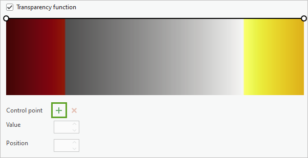
Two additional points are added to the symbol range.
Click the first control point and set Value to 100 percent and Position to 3 percent.
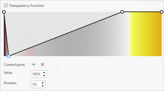
For the second control point, set Value to 100 percent and Position to 80 percent.
The voxel layer shows areas of high (yellow) and low (red) dissolved oxygen in the Caribbean Sea.
On the Quick Access Toolbar, click Save to save the project.

You've added the EMU NetCDF file as a multidimensional voxel layer in a local scene in ArcGIS Pro. Next, you'll visually analyze the voxel layer by defining surfaces and making basic changes to the voxel layer appearance such as selecting a variable and changing stretch parameters.

Visually analyze the EMUs in 3D

Previously, you loaded the EMU NetCDF file as a voxel layer in ArcGIS Pro. Next, you'll create surfaces such as isosurfaces and sections to visually analyze variables.

Create an isosurface

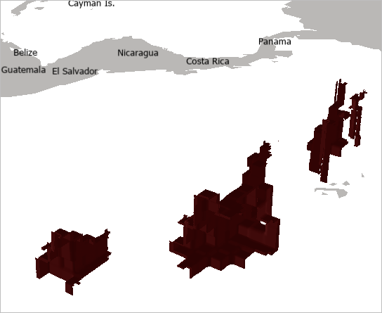
First, you'll define an isosurface at a specific value to visually analyze the distribution of dissolved oxygen. An isosurface describes a surface within the voxel layer along a specified value. For example, an isosurface of dissolved oxygen at 2.85 microliters/liter shows all the places in the Caribbean Sea with that value which can happen at different depths.

In the Contents pane, under EMU_Caribbean_Voxel, click mole_concentration_of_dissolved_molecular_oxygen_in_sea_water two times.
The field becomes editable.
Name the variable Concentration of Dissolved Oxygen.
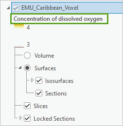
Expand and select Surfaces.
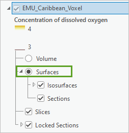
The voxel will be removed from the map since you haven't created a surface yet.
Under Surfaces, right-click Isosurfaces and select Create Isosurface.

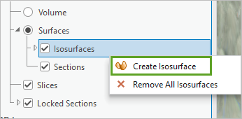
A new isosurface is created within the voxel layer, and the Voxel Exploration pane appears.
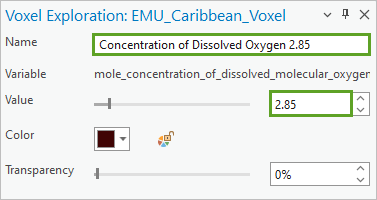
In the Voxel Exploration pane, for Name, type Concentration of Dissolved Oxygen 2.85. For Value, type 2.85.

An isosurface at 2.85 microliters/liter of dissolved oxygen is drawn on the map.
Next, you will update the Vertical Exaggeration for the voxel and Ground Elevation Surface.
Note:
See Change the appearance of a voxel layer to learn more about configuring voxel data to be positioned correctly with respect to the bathymetry.
In the Contents pane, turn on the World Ocean Base and WorldElevation3D/TopoBathy3D layers.
In the Contents pane, click Ground.
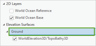
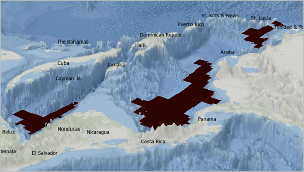
On the ribbon, in the Elevation Surface Layer tab, in the Drawing group, for Vertical Exaggeration, type 40 and press Enter.
On the Contents pane, click the EMU_Caribbean_Voxel layer. On the ribbon, in the Voxel Layer tab, for Elevation, set Vertical Exaggeration to 40.
Right-click the EMU_Carribbean_Voxel layer and click Properties.
In the Layer Properties window, click the Elevation tab and for Exaggeration mode, choose Z-coordinates and click OK.

Create a section

Next, you'll visually explore variables by defining sections that span across the voxel layers. You'll define a section, then dynamically change its position, tilt, and orientation. The new section will be locked to be visible together with other variables.

On the ribbon, on the Voxel Layer tab, in the Variable group, choose sea_water_temperature.
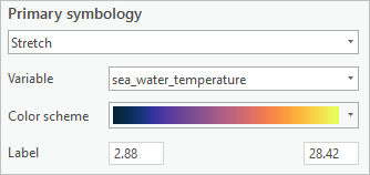
In the Drawing group, click Symbology. In the Symbology pane, for Color scheme, check Show Names and choose Thermal.
In the Contents pane, uncheck the Countries layer.
On the ribbon, click the Data tab. In the Explore group, choose Slice and Section.
The Slice and Section toolbar appears at the bottom of the scene.
In the Slice and Section toolbar, select Vertical Section.
On the map, click a point on the northwest coast of Nicaragua to start the slice then double-click the second point off the coast of the Yucatan peninsula.

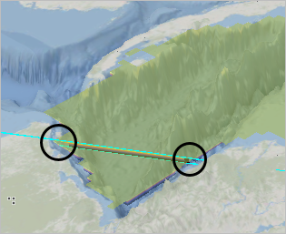
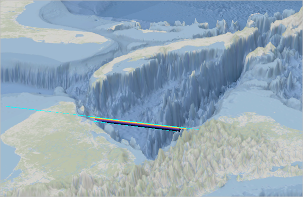
A new vertical section is added to the scene.
In the Contents pane, right-click Section 1 and choose Lock Section.
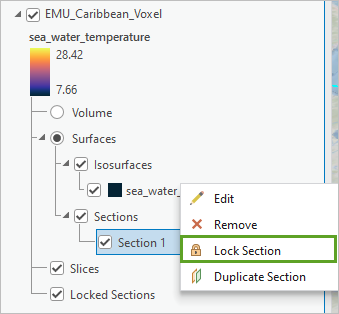
The locked section moves into the Locked Sections group of the voxel layer. The section is now a snapshot at the defined location and can be viewed even if a different variable is selected. This allows you to explore different variables together.
On the ribbon, on the Voxel Layer tab, in the Variable group, choose the mole_concentration_of_dissolved_molecular_oxygen_in_sea_water variable.
The Concentration of Dissolved Oxygen 2.85 isosurface and the sea water temperature section appear on the scene.
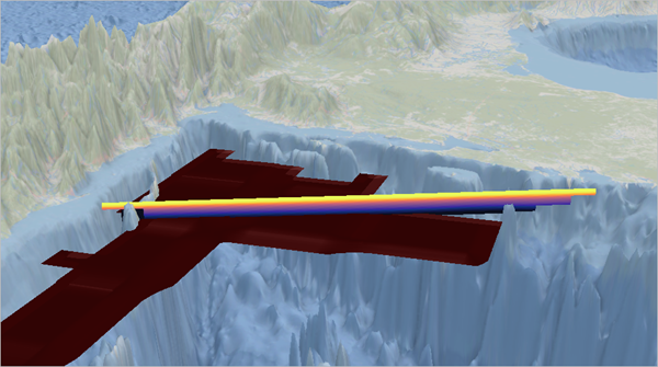
The example image shows a Sea Water Temperature cross section from Nicaragua to the Yucatan peninsula. It also shows an isosurface of Dissolved Oxygen for values of 2.85 microliters/liter.

In this lesson, you created a NetCDF file using Python notebooks in ArcGIS Pro. You downloaded the EMU point feature class and loaded its values into the new EMU NetCDF file. You loaded and visually analyzed this NetCDF file in 3D as a multidimensional voxel layer in a local scene.

You can find more tutorials in the tutorial gallery.

Create a NetCDF file Use an ArcGIS Notebook in ArcGIS Pro to create a NetCDF file of the world's Ecological Marine Units (EMU) dataset.	30 minutes
Add a NetCDF file as a voxel layer Add the EMU NetCDF file as a multidimensional voxel layer in a local scene in ArcGIS Pro.	10 minutes
Visually analyze the EMUs in 3D Display EMU variables such as sea water temperature, salinity, or dissolved oxygen in a 3D voxel layer.	20 minutes

Create a NetCDF file

Add a NetCDF file as a voxel layer

Visually analyze the EMUs in 3D

Set up a new project

Note:

Note:

Create an empty NetCDF file

Note:

Note:

Note:

Load data into the NetCDF file

Tip:

Add a multidimensional voxel layer

Note:

Create an isosurface

Note:

Create a section

The Science of Where: A voxel visualization of smoke plume rise and dispersion

3D Visualization and Analytics Fundamentals

Creating 3D Features from Existing Data

Requirements

Outline

Create a NetCDF file

Add a NetCDF file as a voxel layer

Visually analyze the EMUs in 3D

Create a NetCDF file

Set up a new project

Note:

Note:

Create an empty NetCDF file

Note:

Note:

Note:

Load data into the NetCDF file

Tip:

Add a NetCDF file as a voxel layer

Add a multidimensional voxel layer

Note:

Visually analyze the EMUs in 3D

Create an isosurface

Note:

Create a section

Acknowledgements

Send Us Feedback

Share and repurpose this tutorial

Ready to learn more?

Related Esri training

The Science of Where: A voxel visualization of smoke plume rise and dispersion

3D Visualization and Analytics Fundamentals

Creating 3D Features from Existing Data