Site a sustainable shrimp farm

In recent years, Costa Rica has been developing organic and sustainable shrimp farming. In particular, it is trying to move the production away from mangrove forests, as intensive shrimp farming is destructive to that environment. It also encourages a practice that does away with the heavy use of chemicals and antibiotics. As the new approach to shrimp farming is increasingly successful, local farmers are looking for potential locations for new organic and sustainable shrimp farms. In this tutorial, you'll use the ArcGIS Pro Suitability Modeler to locate new potential farming sites in the Gulf of Nicoya, Costa Rica, based on several criteria. You'll generate a suitability map indicating the most favorable areas based on the criteria. Then, from the suitability map, you'll identify the five best potential shrimp locations.

This tutorial was last tested on January 26, 2025, using ArcGIS Pro 3.4. If you're using a different version of ArcGIS Pro, you may encounter different functionality and results.

Requirements

• ArcGIS Pro (see options for software access)
• ArcGIS Spatial Analyst extension

Understand the context and method

First, you'll learn a bit about shrimp farming and then about the criteria you'll use in this suitability analysis.

Intensive shrimp farming

Shrimp farming around the world is a large industry and the market for farmed cheap shrimp is growing each year. As world consumption has risen and costs have gone down, commercial shrimp farming has grown rapidly in many countries around the world. Shrimp farming mainly takes place along the coast where briny water is used to fill ponds where shrimp are raised. Traditionally, ponds are established in locations where mangrove forests are located and as a result, commercial farming destroys mangroves that serve as natural nurseries for wild shrimp and act as a buffer to sea level rise.

In the forefront of this photograph, the ponds of a shrimp farm in Costa Rica (image: Adobe Stock).

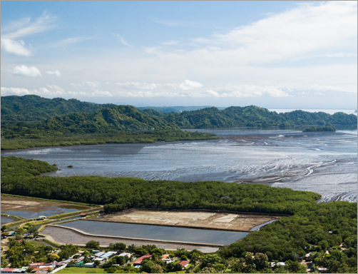
Often, to boost production, farmers increase shrimp density in ponds, apply antibiotics and pesticides to reduce shrimp mortality, and kill algae resulting from high nitrates that develop as a result of the high density and feeding regimen. Shrimp in these farms are basically living on top of each other in their own waste. In these cases, before harvesting, ponds are drained of chemicals, and antibiotic-laced water is pumped into the rivers and canals that flow into the surrounding sea. For a few weeks, the shrimp are kept in clean ponds to clear chemicals from their system and then they are harvested and shipped to consumers around the world.

Shrimp farming in Costa Rica

Costa Rica has abundant freshwater resources, and includes mountain ranges, a tropical climate, and a marine exclusive economic zone of almost 600,000 square kilometers. This makes the country suitable for aquaculture development and ideal for shrimp production.

Initial shrimp production from 2009 to 2015 was associated with the presence of diseases, farmers with a low level of technical skills, few environmental policies, little local trade, and strong competition from South East Asian sources. However, since 2018, the industry has developed an organic supply chain that has achieved certification under the European organic regulations. Many large-scale operators and most small farmers have joined the initiative and are now operating organic shrimp farms.

As a result, within Costa Rica, an organic production protocol was developed, organic nauplii (shrimp larvae) and feed were organized, and some hatcheries converted to organic production. Farmers have been trained in organic production and are now producing, selling, and marketing organic shrimp. As the organic market is growing significantly, it is logical to assume that local farmers, many of whom rely on fishing and tourism for a livelihood, would want to establish new farms and ponds to take advantage of the world interest and demand for sustainably farmed organic shrimp.

Suitability model

You'll use the ArcGIS Pro Suitability Modeler to locate new potential farming sites in the Gulf of Nicoya, Costa Rica.

A view of the Gulf of Nicoya is shown (image: Adobe Stock).

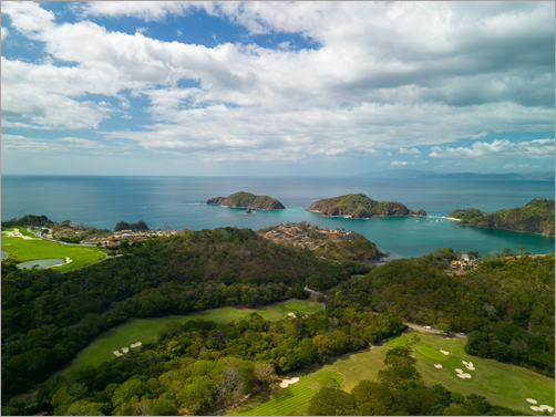
Developing a suitability model is a well-known GIS approach to identify the best locations for a site based on several criteria. In this tutorial, you'll use the following five criteria to find the most suitable locations for organic shrimp farms:

• Be in close proximity to salt water, which is needed to grow shrimp. In this context, this means being close to the Gulf of Nicoya, which opens to the Pacific Ocean.
• Be on specific land use types: the most suitable is land currently covered by grassland, shrubland, or used for agriculture purposes. Mangrove forests should be completely avoided.
• Be in close proximity to the road network to get the shrimp to processing plants and market.
• Be located near rivers to flush shrimp ponds regularly with fresh water.
• Be located on relatively flat grounds, as steep slopes are not suitable to set up shrimp ponds.

Using the ArcGIS Pro Suitability Modeler, you will do the following:

• Generate a suitability map indicating the most favorable areas based on the five criteria.
• From the suitability map, identify the five best potential shrimp locations.

There are five main steps for creating a suitability model:

• Determine and prepare the criteria data.
• Transform the values of each criterion to a common suitability scale.
• Weight the criteria relative to one another and combine them to create a suitability map.
• Locate the areas that best match your criteria.

So far, you learned about shrimp farming in Costa Rica and reviewed the criteria that you'll use in the suitability model to locate new potential farming sites in the Gulf of Nicoya.

Explore shrimp farm suitability data

You will now download a project that contains all the data for this tutorial and open it in ArcGIS Pro. You'll then explore the data layers.

Get started

You will download the project package.

1. Download the ShrimpFarm package.

   A file named ShrimpFarm.ppkx is downloaded to your computer.

   Note:

   A .ppkx file is an ArcGIS Pro project package and may contain maps, data, and other files that you can open in ArcGIS Pro. Learn more about managing .ppkx files in this guide.

2. Locate the downloaded file on your computer.

   Tip:

   In most web browsers, it is downloaded to your computer's Downloads folder by default.

3. Double-click ShrimpFarm.ppkx to open it in ArcGIS Pro. If prompted, sign in with your ArcGIS account.

   Note:

   If you don't have access to ArcGIS Pro or an ArcGIS organizational account, see options for software access.

   The project opens to display the Gulf of Nicoya map.

   

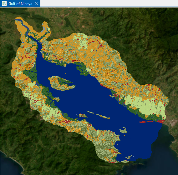
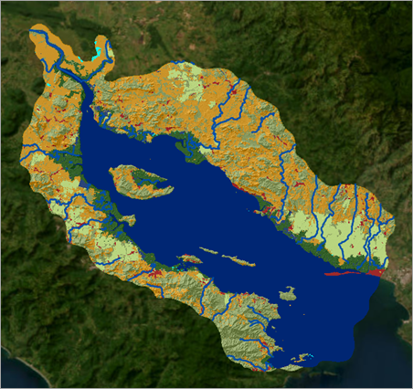
   The map currently displaying includes a Land_Cover layer, a Hillshade layer underneath giving a sense of the region's elevation, and the gulf water body, represented in dark blue (Gulf_Water). The background is the World Imagery basemap.

4. Review the Contents pane.

You can see that several other layers are included, all relevant to the suitability analysis you will perform in the tutorial. You'll now examine those layers.

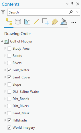
Note:

All source data layers have been clipped to the extent of the Land_Mask area, which represents the land within the study area. For more information, see the Apply this workflow to your own data section at the end of this tutorial.

Explore the criteria layers

You'll start by exploring the Land_Cover layer, which is already turned on.

1. In the Contents pane, click the arrow next Land_Cover to expand the layer legend.

   

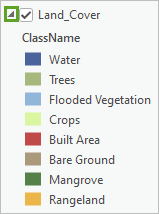
   This layer contains various types of land cover categories. Some categories are more suitable for shrimp farming than others and at varying degrees. Rangeland (mostly grassland and shrubland) and Crops are most suitable, followed by Bare Ground, Trees, and Flooded Vegetation that are moderately suitable, with Built Area, Water, and Mangrove being the least suitable.

   Note that there are many mangroves (symbolized in darker green) near the coast. A mangrove is a shrub or small tree that grows in coastal saline or brackish water. It is salt-tolerant and adapted to life in harsh coastal conditions. Mangrove forests act as buffers from cyclones and are important to mitigate the impact of climate change. As mentioned, the Costa Rican government wants to protect mangroves and move shrimp farming activities out of them.

   Note:

   Land cover rasters are usually derived from multispectral imagery, using image classification techniques to determine the cover types, based on their spectral signatures. Check out the tutorial Calculate impervious surfaces from spectral imagery for an example of such a classification workflow. In turn, the Gulf_Water layer was derived from the land cover layer.

2. On the map, zoom in and out with the mouse wheel button to explore the Land_Cover layer.
3. When you are finished, in the Contents pane, collapse the Land_Cover layer. Right-click the Land_Cover layer and choose Zoom To Layer to go back to the entire study area.

   

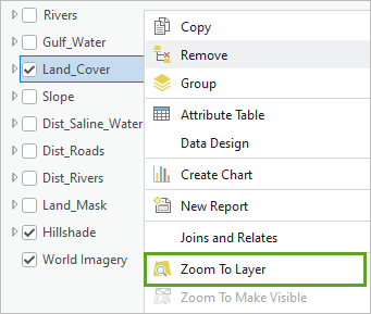
4. Click the box next to Gulf_Water to turn the layer off and back on and better visualize its extent.

   

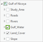
   Salt water is needed to fill the ponds where the shrimp are grown. As salt water can be found in the gulf, your suitability model needs to ensure that the new farm sites are as close as possible to the gulf coast (while still avoiding the protected mangroves). Next, you'll become familiar with the road network.

5. In the Contents pane, turn on the Roads layer. Explore the layer symbolized in dark gray.

   

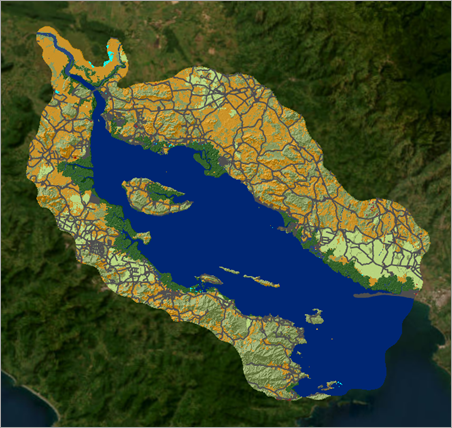
   Shrimp farmers need to get their shrimp to processing plants and markets for sale and redistribution. As a result, sites with access to the road network are preferred.

6. When you are finished exploring, in the Contents pane, turn off the Roads layer.
7. In the Contents pane, turn the Rivers layer on. Explore the layer, symbolized in medium blue.

   

   Shrimp farming requires access to fresh water to flush the ponds regularly, so proximity to a river is highly desirable.

8. When you are finished exploring, in the Contents pane, turn off the Rivers layer.

   Next, you'll explore the Slope layer.

9. In the Contents pane, turn off the Land_Cover layer and turn on the Slope layer.

   

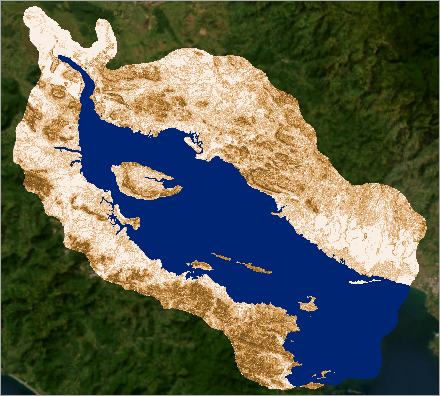
   The layer is a raster representing the slope incline, from 0 to 90 degrees, for every cell in the study area. It is symbolized in white (flatter areas) to brown (steeper slopes). Shrimp ponds must be located on relatively flat grounds, so steep slopes are not suitable.

   Note:

   The slope layer was derived from an elevation data layer, itself derived from remote sensing data. The hillshade layer was also derived from the same elevation data. For more information on how to generate these layers, see the Apply this workflow to your own data section at the end of this tutorial.

10. When you are finished exploring, in the Contents pane, turn off the Slope layer. If necessary, right-click Land_Cover and choose Zoom To Layer.

Next, you will review distance rasters that were derived from some of the layers explored so far.

Explore the distance rasters

In your suitability model, you can use the land cover layer directly, as different suitability levels will be assigned to different land cover types. For instance, Rangeland will have a very high suitability, and Mangrove a very low suitability. Similarly, you can use the slope layer directly.

However, other criteria require that you generate a derived raster layer. For instance, for the salt water criterion, it is not the case that a location exactly on the gulf water is suitable and a location not on the gulf water is unsuitable. Instead, the change in suitability is incremental. The closer a location is to the gulf water, the more suitable it is. The farther away a location is from the gulf water, the less suitable it is. This means that the suitability level of a location depends on how far it is from the gulf. To determine that distance value, you must derive a distance raster, which identifies how far each location within the study area is from the gulf water. Similarly, you also must derive distance rasters for the roads and rivers criteria. Those distance rasters will be used in your suitability model.

This tutorial is not focused on the preparation of the data, so the derived rasters were generated for you.

Note:

To learn more on how to prepare such derived rasters, see the Apply this workflow to your own data section at the end of this tutorial.

You’ll review these layers now.

1. In the Contents pane, identify the three distance rasters, whose names start with Dist_.

   

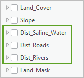
2. Turn on the Dist_Saline_Water layer and expand it.

   

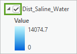
   From the legend, you can see that the different locations in the study area can be from 0 to 14,074.7 meters (or 14.075 kilometers) from the gulf. On the map, verify that the low values (dark blue) are closer to the gulf and the higher values (light blue) are farther away.

   

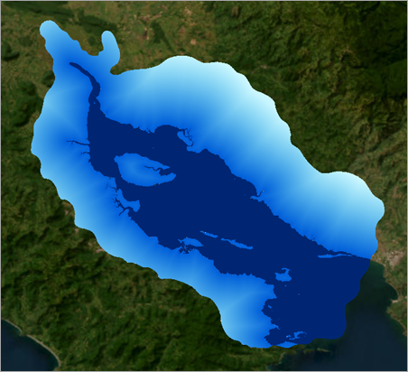
3. Click some of the locations to see the distance value displayed in the pop-up.

   

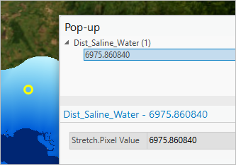
4. Close the pop-up panel. In the Contents pane, collapse the Dist_Saline_Water layer.
5. On your own, review the additional distance layers that represent the following:
   • Distance to roads (Dist_Roads)
   • Distance to rivers (Dist_Rivers)

   You can also turn on the original layers Roads and Rivers to better understand how original and derived layers relate to each other. For instance, compare Dist_Roads and Roads.

   

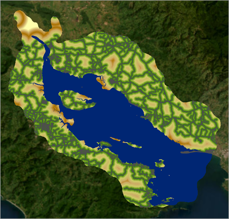
6. Observe how each layer has a different distance range.

   For instance, Dist_Roads ranges from 0 to 5.6 kilometers, and Dist_Rivers varies from 0 to almost 13.9 kilometers. Later, you will need to transform these into a common scale to combine them in your suitability model.

7. In the Contents pane, turn off all distance layers and turn back on the Land_Cover layer.
8. On the Quick Access Toolbar, click the Save button to save the project.

   

   Note:

   A message may warn you that saving this project file with the current ArcGIS Pro version will prevent you from opening it again in an earlier version. If you see this message, click Yes to proceed.

You have now set up the project and explored the criteria layers. Next, you'll create the suitability model.

Develop the suitability model and transform the layers

Now that you have explored the shrimp farm suitability criteria and layers, you are ready to begin creating a suitability model using the Suitability Modeler to identify the five best potential sites for new shrimp farms.

The basic premise behind the Suitability Modeler is that constructing a model is an iterative, dynamic process. To generate the model, you will interact with panes, plots, and maps and receive immediate feedback that will help you make decisions, such as defining model parameters, and seeing how those decisions will affect the final results.

The general steps to create a suitability model are the following:

• Identify criteria.
• Transform the values within each criterion onto a common scale.
• Weight the criteria relative to one another and combine them to create a suitability map.
• Locate the areas that best match your criteria.

Create the model and add the criteria

You'll start with creating the model and adding the criteria to it.

1. On the ribbon, on the Analysis tab, in the Workflows group, click Suitability Modeler.

   

   The Suitability Modeler pane appears. Note the Settings, Suitability, and Locate tabs: you will use all three in this workflow.

   

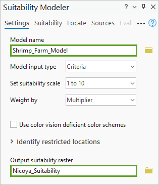
2. In the Suitability Modeler pane, confirm that the Settings tab is active and set the following parameters:
   • For Model Name, type Shrimp_Farm_Model.
   • For Output suitability raster, type Nicoya_Suitability.
   • Accept all other default values.

   

   Note:

   By default, the Suitability Modeler uses a set of color schemes that are intended for users with unimpaired color vision. The default color schemes will be used in this tutorial. However, if desired, the Use color vision deficient color schemes option is available to enable color vision deficient (CVD) color schemes for all maps, legends, and charts.

   You’ll save the model.

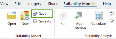
3. On the ribbon, on the Suitability Modeler tab, in the Suitability Model group, click Save.

   

   Note:

   If you need to take a break and close ArcGIS Pro, you can always access this model again later on. Open the Suitability Modeler pane, and click the Browse button near the model's name. Browse to Folders > ShrimpFarm > ShrimpFarm.sam > ShrimpFarm and click OK. Then continue from where you left off.

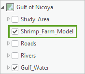
4. In the Contents pane, confirm that a new group layer named Shrimp_Farm_Model has been added.

   It is currently empty.

   

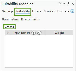
5. In the Suitability Modeler pane, click the Suitability tab.

   This tab contains a Criteria table. You'll add the criteria for the model to the table.

   

   As a reminder, the following are the five criteria defining the most suitable locations for organic shrimp farms:

   • Be in close proximity to salt water, that is, to the Gulf of Nicoya.
   • Be on specific land use types: the most suitable is land currently covered by grassland, shrubland, or used for agriculture purposes. Mangrove forests should be completely avoided.
   • Be in close proximity to the road network to get the shrimp to processing plants and market.
   • Be located near rivers to flush shrimp ponds regularly with fresh water.
   • Be located on relatively flat grounds, as steep slopes are not suitable to set up shrimp ponds.
6. In the Suitability Modeler pane, under Criteria, next to Input Rasters, click the Add raster criteria as layers from the Contents list button.

   

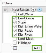
7. In the Criteria layer list, click the check boxes for the following layers:
   • Land_Cover
   • Slope
   • Dist_Saline_Water
   • Dist_Roads
   • Dist_Rivers
8. In the Criteria layer list, click Add.

   

9. In the Suitability Modeler pane, for Criteria, confirm the five criteria layers have been successfully added to the list.

   

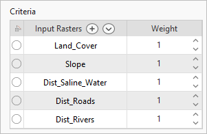
   Note:

   If you added a layer by mistake, you can hover over its name in the Criteria table and click the red arrow to remove it.

10. In the Contents pane, confirm that the Shrimp_Farm_Model group layer is turned on and expanded and that the five criteria layers have also been successfully added to it.

    

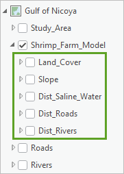
    This group layer stores all the layers relevant to the model, and more will be added as you progress through the workflow.

In this section, you created a suitability model and added five criteria layers to it.

Learn about different types of rasters

To prepare for the next steps of the workflow, you will learn about different types of rasters.

In your suitability model, you will combine all the criteria. But before that, you must convert each criterion to a common 1-to-10 suitability scale, so that they can all contribute equally to the model. The most preferred value within a criterion is assigned a 10, and the least desirable value a 1. This transformation can be done differently based on the raster type and criterion's meaning.

One important raster type distinction is between continuous and categorical rasters. For instance, Dist_Saline_Water is a continuous raster—it has a numeric value range that represents distances from 0 to 14,344.8 meters, and its cells can take any decimal value within that range. Similarly, Slope, Dist_Roads, and Dist_Rivers are also continuous rasters. In contrast, Land_Cover is a categorical raster—its cells have values that represent categories, such as Mangrove or Grassland, and there are only eight possible categories for that raster.

Note:

In continuous data, the values have meaning relative to one another. For instance, a distance of 50 meters from a road is half as far as a distance of 100 meters. Within categorical data, you don't have those types of relationships between values. A land use of 1 (Water) is not half the land use assigned a 2 (Trees).

Continuous rasters are generally represented with floating-points and categorical rasters with integers.

The transformation for continuous and categorical rasters will be handled differently. You will also learn about two ways of transforming continuous rasters, based on the specific data they represent: applying a continuous function or a range of classes.

Layer name	Type	Transformation method
Dist_Saline_Water	Continuous	Continuous function
Land_Cover	Categorical	Unique categories
Dist_Roads	Continuous	Range of classes
Dist_Rivers	Continuous	Continuous function
Slope	Continuous	Continuous function

Transform continuous data

You'll start with transforming the continuous raster Dist_Saline_Water. You'll do that by applying a continuous function.

1. In the Suitability Modeler pane, under Criteria, click the circle next to the Dist_Saline_Water criterion.

   

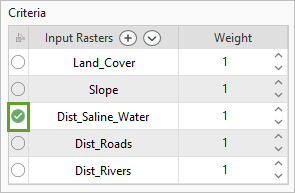
   The circle turns green and the Transformation pane appears.

2. If necessary, resize and reposition the Transformation pane below the Gulf of Nicoya map, so you can see both the pane and the map, as shown in the following example image.

   

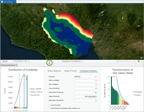
   In the Contents pane, in the Shrimp_Farm_Model group layer, two additional layers were also added: Nicoya_Suitability and Transformed Dist_Saline_Water.

   

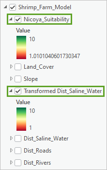
   The Transformed Dist_Saline_Water layer shows the Dist_Saline_Water layer transformed to a 1-to-10 scale. For now, it is using a default transformation. The Nicoya_Suitability layer will show the combination of all the transformed criteria layers as you activate them. At the moment, there is only one transformed layer, so Nicoya_Suitability is a duplicate of Transformed Dist_Saline_Water.

3. Confirm that Transformed Dist_Saline_Water is turned on, and turn off Nicoya_Suitability.

   You'll use the Transformation pane to refine the transformation applied to the Dist_Saline_Water layer.

4. Review the content of the Transformation pane.

   

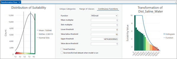
   The Transformation pane has three sections, which all provide information to assist you with selecting the most appropriate transformation. The center section is used to specify the transformation method.: Currently, the MSSmall function is used. The section on the right displays a transformation plot, and the section on the left displays a suitability plot.

5. In the Transformation pane, on the Continuous Functions tab, click the Function drop-down list and review the available functions. Confirm MSSmall is currently selected.

   

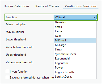
   Since the Dist_Saline_Water layer is a continuous raster, the Continuous Functions method MSSmall was applied by default. Depending on your specific data, other continuous functions listed in the drop-down list may be more appropriate.

6. Observe the Transformation of Dist_Saline_Water plot.

   

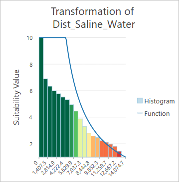
   The plot shows how the values of the original raster (x axis) are transformed into 1-to-10 suitability values (y axis). The transformation function is displayed as a blue line. For instance, you can see that the original value of 5,629.9 (meters) is transformed into a suitability of about 5. Applying a continuous function means that with each meter you move away from the gulf, the preference continuously decreases, with the closer distances being more desirable. With the MSSmall function, the closer distances receive the highest suitability (a value of 10) and then after about 4,500 meters, the preference sharply decreases.

   The bars of the plot show a histogram indicating the relative number of cells for the different value ranges on the x axis. The bar colors correspond to suitability: green is most preferred and red least preferred.

7. Look at the Transformation of Dist_Saline_Water layer on the map.

   

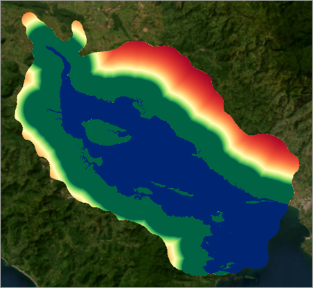
   The same color symbolization is applied on the plot and on the map.

8. On the map, click several locations in the area of interest to see their value in the Pop-up pane.

   As expected, they vary from 1 to 10.

9. Close the Pop-up pane.
10. In the Transformation pane, review the Distribution of Suitability plot.

    

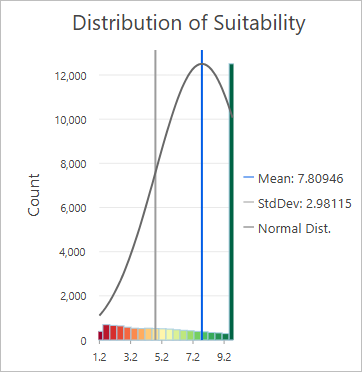
    This histogram shows the distribution of suitability values in the combined suitability layer: the x axis shows the range of suitability values (currently 1 to 10), and the y axis shows how many cells were assigned to each value. The histogram and suitability map are updated with each change in the model. They provide feedback on how changes in each criterion transformation will affect the final output.

    You'll now explore different transformations that can be applied to Dist_Saline_Water.

11. In the Transformation pane, for Function, choose Linear.

    The two plots and the map update.

12. Review the Transformation of Dist_Saline_Water plot.

    

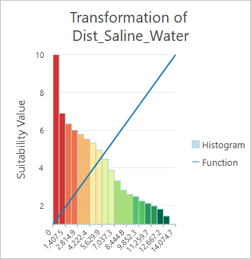
    In the plot, the blue line now shows the progression of a typical linear function. The locations closer to the water are now less preferred and the preference increases as you move away from the water. This is not what you want, so you'll invert the transformation.

13. In the Transformation pane, check the Invert function box.

    

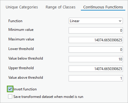
    The transformation is now back in the right direction (lower distances are preferred). The main difference with the MSSmall transformation is that the suitability values drop more steadily (linearly).

14. Look at the map to see how the MSSmall and Linear transformations change the Transformed Dist_Saline_Water layer.

    You can go back and forth between the functions a few times.

15. In the Transformation pane, using the Function drop-down list, explore some of the other functions to see their effect.

    MSSmall is a good choice for this layer. The suitability sharply decreases as the distance from the coast increases. However, the sharp drop needs to happen sooner, because the shrimp farm should be located close to the coast for easy access to briny water. You'll achieve this with the Mean multiplier parameter.

16. In the Transformation pane, for Function, select the MSSmall function.
17. For Mean multiplier, type 0.2, and press Enter.

    

    The sharp drop now happens much sooner both on the transformation plot and the map. Areas very close to the ocean are most preferred (green), while farther areas quickly drop to less preferred values (yellow and red).

    

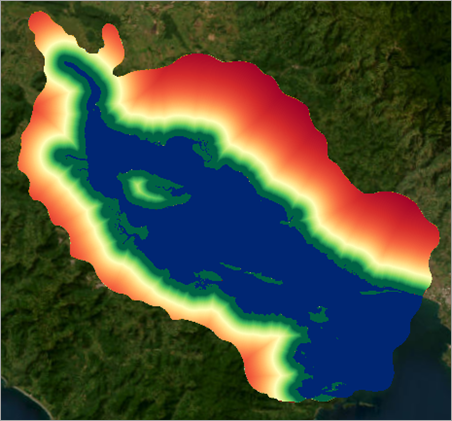
In this section, you saw how the Suitability Modeler allows you to receive dynamic feedback on your transformation choices, with a focus on continuous functions. In the next section, you'll explore categorical transformations.

Transform unique categories

Now, you'll transform the second criterion, Land_Cover, onto the common 1-to-10 scale. Certain land cover types are more suitable to develop shrimp ponds than others.

1. In the Suitability Modeler pane, for Criteria, click the circle next to Land_Cover.

   

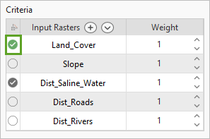
   Note:

   The button turns green, indicating it is the active criterion in the Transformation pane. The button turns gray once the criterion has been transformed and is no longer active in the Transformation pane.

   The Transformation and Contents panes update.

2. In the Contents pane, review the Shrimp_Farm_Model group layer.

   An additional layer named Transformed Land_Cover has been added. The Nicoya_Suitability layer has now a range from 2 to 20, as it combines the first two criteria.

3. Ensure that Transformed Land_Cover is turned on. Turn off all other layers in the Shrimp_Farm_Model group layer.

   

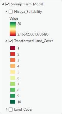
4. Review the Transformation pane.

   Since Land_Cover is categorical data, the Unique Categories transformation method has been applied by default, and proposed transformation values are listed in a table.

5. In the Transformation pane, for Field, choose Class_Name.

   

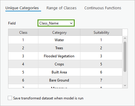
   The table updates to show the name of every land cover type in the Category column. The Class column indicates the numeric value corresponding to each land cover type. The Suitability column shows the result of the one-to-one transformation method that was applied. Each land cover category is assigned a suitability value, based on how preferred it is for developing a shrimp farm. For now, the suitability values have been assigned in the order the classes are listed. Next, you'll enter your desired values.

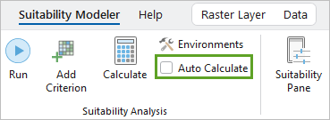
   You'll turn off Auto Calculate to prevent the Suitability Modeler from applying immediate updates each time you change a value.

6. On the ribbon, on the Suitability Modeler tab, in the Suitability Analysis group, uncheck Auto Calculate.

   

7. In the Unique Categories table, update the Suitability value for each Category.

   Use the following table to assign the desired suitability values.

   Category	Suitability
   Water	1
   Trees	4
   Flooded Vegetation	3
   Crops	6
   Built area	1
   Bare Ground	5
   Mangroves	1
   Rangeland	9

   The most suitable land cover types, such as Rangeland and Crops are assigned the higher values, and the least suitable are assigned the lowest values.

8. On the ribbon, on the Suitability Modeler tab, in the Suitability Analysis group, click Calculate and check Auto Calculate.

   

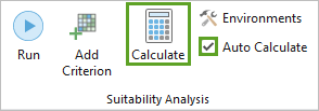
   The new suitability values have now been applied to the Land_Cover types, and subsequent calculations will now be applied automatically when a change is made to the model parameters. You'll inspect the updated plots and layers.

9. In the Transformation pane, review the updated Transformation of Land_Cover bar chart.

   

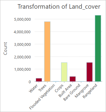
   The colors on the transformation bar chart depict the suitability preference for each land use type, from green (most preferred) to red (least suitable). The height of the bars indicates the number of raster cells for each land use. Taller bars indicate that the land use type is more common within the study area.

10. On the map, examine the Transformed Land_Cover layer.

    

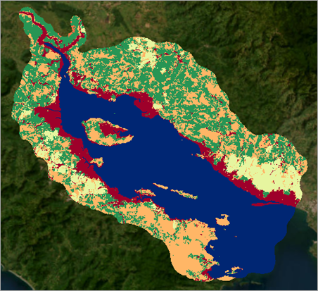
    Notice the red areas along the coast. They represent mangrove forests and some urban areas and are the least suitable. Tree-covered areas (in orange) are not very suitable. In contrast, rangeland and crops are most suitable (in dark and light green).

11. In the Transformation pane, observe the updated Distribution of Suitability plot.

    

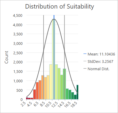
    The suitability plot shows the distribution of the combined suitability with the first two criteria. The value range on the x axis is now a maximum of 2 to 20, because the 1 to 10 ranges for the two activated criteria are summed up. The medium suitability (in pale green) is currently the most often assigned.

12. In the Contents pane, in the Shrimp_Farm_Model group layer, turn on the Nicoya_Suitability layer.

    

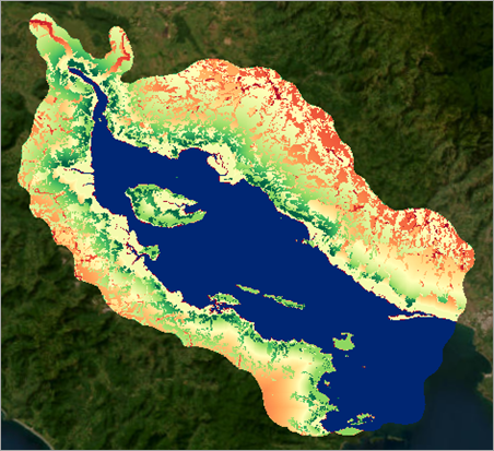
    The suitability map is now a combination of the first two transformed criteria layers.

13. Turn off the Nicoya_Suitability layer.
14. On the ribbon, on the Suitability Modeler tab, click Save to save the model.
15. Press Ctrl+S to save the project.

    Note:

    Model and project are saved independently from each other, so these last two instructions are necessary.

Transform a range of classes

Next, you will transform the third criterion, distance to roads.

1. In the Suitability Modeler pane, for Criteria, click the circle next to the Dist_Roads criterion.

   

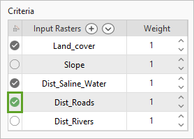
   As usual, the Transformation pane and the Contents pane update.

2. In the Contents pane, in the Shrimp_Farm_Model group layer, confirm that Dist_Roads is on, and turn off all of the other layers in the group layer.
3. Review the Transformation pane.

   Since Dist_Roads is a continuous raster, the continuous function MSSmall was applied by default. However, the cost to get shrimp to processing plants using the roads does not change with each meter traveled. Instead, the costs can be grouped into distance groups of equal cost, and each range will be assigned a single suitability value.

4. In the Transformation pane, click the Range of Classes transformation tab.

   

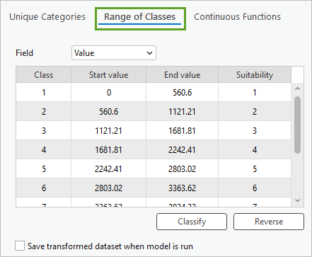
   The range of distance-to-roads values is now divided into 10 classes. The first class is for distances from about 0 to 560 meters; the second class, 560 to 1121 meters; and so forth.

5. Review the Transformation of Dist_Roads plot.

   

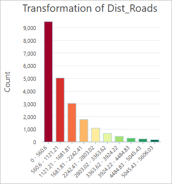
   You can see that currently the closest distances are the least preferred and appear in red. This is the reverse of what you want, so you'll invert the suitability assignment.

6. In the Transformation pane, on the Range of Classes tab, click the Reverse button.

   

   The plots and the map are updated to the desired effect.

7. In the Transformation pane, review the updated Transformation of Dist_Roads plot.

   Distances close to the roads are now classified as most suitable (green).

8. In the Contents pane, drag the Roads layer above the Shrimp_Farm_Model group layer and turn it on. Confirm that Transformation of Dist_Roads is on, and turn off all other layers in the Shrimp_Farm_Model group layer.

   

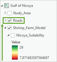
   The roads now display on top of the Transformed Dist_Roads layer.

9. On the map, examine the Transformed Dist_Roads and Roads layers.

   

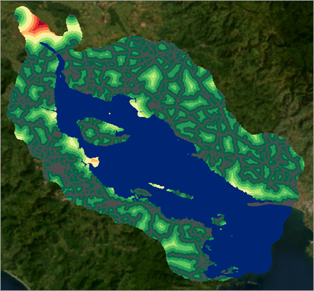
10. Zoom in to verify that the distance values are grouped into 10 classes of distinct ranges around the location of roads.

    

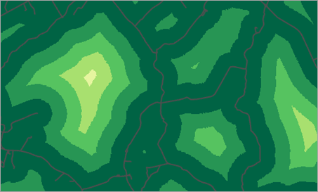
    The range closest to the roads is the greenest because it is the most suitable.

11. In the Contents pane, turn off the Roads layer. In the Shrimp_Farm_Model group layer, turn on the Nicoya_Suitability layer and zoom out to the Nicoya_Suitability layer extent.

    Note:

    During this exploratory stage of the model creation, the Suitability Modeler only processes data within the current extent displayed on the screen. Make sure that you are not zoomed in and that the entire study area appears on the map.

    

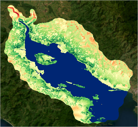
    The suitability map now shows the combination of the first three criteria. The same is true for the Distribution of Suitability plot, which now ranges from about 8 to 30.

    Note:

    The reason lower values (3 to 7) are not represented is that there are no locations in the extent that have the lowest possible values for distance to salt water, land cover, and distance to roads, all at the same time.

12. In the Contents pane, turn off the Nicoya_Suitability layer.
13. Save the model.
14. Save the project.

Transform using the power function

The fourth criterion is the distance to rivers. Before transforming this criterion, you’ll explore some additional functionality of the Suitability Modeler. You'll open two maps side-by-side to view both the current criteria transformation and combined suitability layer at the same time. This will give you even more feedback on the impact of your choices.

1. Click the Gulf of Nicoya map tab to select it.

   

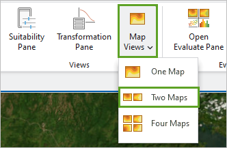
2. On the ribbon, on the Suitability Modeler tab, in the Views group, click the Map Views button and choose Two Maps.

   

   A second map, Suitability-TopRight, appears. The Shrimp_Farm_Model suitability group layer is copied to the Contents pane of the second map.

3. If necessary, position and dock the Suitability-TopRight map pane to the right of the Gulf of Nicoya map, as shown in the example image.

   

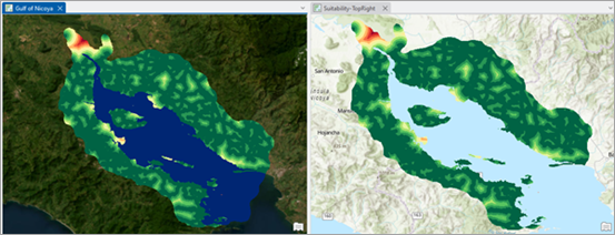
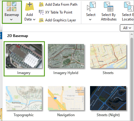
4. Click the Suitability-TopRight map pane to select it. On the ribbon, on the Map tab, in the Layer group, click Basemap and choose Imagery to change the basemap.

   

5. Select the Gulf of Nicoya map pane, and turn off the Gulf_Water layer, so that the two maps look completely similar.
6. For the Gulf of Nicoya map pane, turn on the Nicoya_Suitability layer.
7. If necessary, for each map, zoom to the Nicoya_Suitability layer extent.

   

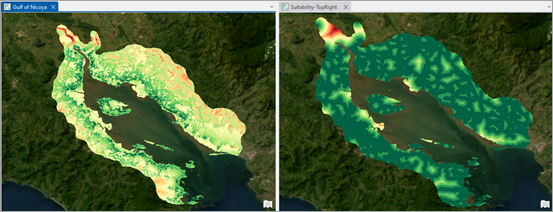
   You can now see at a glance the combined suitability layer on the left and the current transformation map on the right (Transformed Dist_Roads). Next, you'll examine the transformation for the Dist_Rivers criterion.

8. In the Suitability Modeler pane, in the Criteria table, check the circle next to the Dist_Rivers criterion.

   

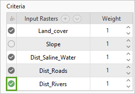
   Since the Dist_Rivers raster is continuous data, as expected, the continuous function MSSmall is applied by default.

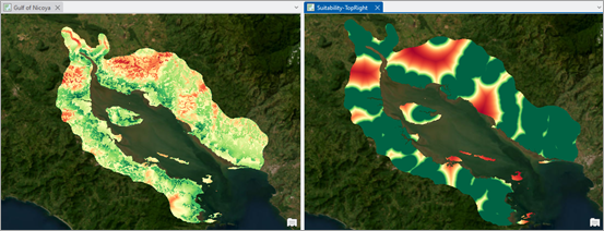
9. Click the Suitability-TopRight map to select it. In the Contents pane, confirm that the Transformed Dist_Rivers layer is on and turn off all the other layers under Shrimp_Farm_Model.

   The Gulf of Nicoya map pane now displays the Nicoya_Suitability layer combining the four activated criteria, while the Suitability-TopRight map pane displays the Transformed Dist_Rivers layer.

   

10. In the Transformation pane, review the current transformation plot.

    

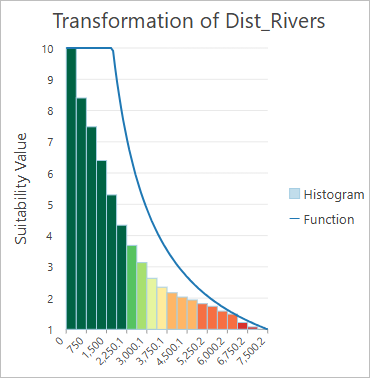
    Notice that, with the MSSmall function, the distance up to around 2,250 meters is considered most suitable and then the suitability sharply declines. This does not capture the desired suitability, because the shrimp farm should be very close to a river for easy access to fresh water. Instead, you'll use the Power function.

11. In the Transformation pane, on the Continuous Functions tab, for Function, select the Power function.

    

12. In the Transformation pane, review the updated transformation plot.

    

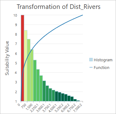
    The locations closer to the rivers are less preferred when the Power function is first applied. You must invert it.

13. In the Transformation pane, on the Continuous Functions tab, check the Invert function box.

    

    The plots and the maps update.

14. In the Transformation pane, review the updated transformation plot.

    

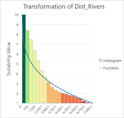
    The locations very close to rivers (in green) are now highly preferred, and then the preference drops quickly and eventually tapers down. The inverted Power function captures the desired suitability transformation.

    On the Suitability-TopRight map tab, in the Transformed Dist_Rivers layer, now, only the areas very close to the rivers appear in green. On the Gulf of Nicoya map tab, you can see how the distance to rivers influences the combined suitability map. Some of the most suitable areas (in green) are now along the rivers.

    

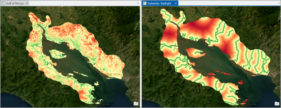
    In the Distribution of Suitability plot, the values now range from about 14 to 37, because it represents four criteria combined.

15. Save the model.
16. Save the project.

Transform the slope

You will now transform the final criterion, the slope.

1. In the Suitability Modeler pane, under Criteria, click the circle next to the Slope criterion.

   

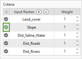
   The Transformed Slope layer shows the Slope layer transformed with the default continuous function MSSmall to a 1-to-10 scale. You will accept this default transformation.

2. In the two maps, observe this last transformed layer and how it influences the combined suitability layer.

   

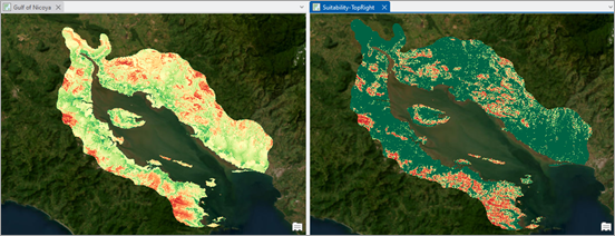
3. On the Suitability-TopRight map tab, turn on the transformed criteria layers one by one, to compare them with the combined Nicoya_Suitability layer on the Gulf of Nicoya map tab.

   Observe how each one has influenced the final suitability map.

   The suitability map now combines all five criteria and ranges from about 17 to 47. You can see clearly that the most suitable areas (in vibrant green) are close to the gulf, but not on mangroves, urban land, or steep slopes, and they tend to be close to rivers. The proximity to roads is harder to see at a glance, but it is taken into account.

4. Save the model.
5. Save the project.

In this part of the workflow, you created a suitability model using the Suitability Modeler, and you transformed all your criteria onto the common scale of 1 to 10.

Complete the suitability analysis

You will now perform the last steps of the analysis to identify the most suitable locations for new sustainable shrimp farms.

Define restricted locations

Because Costa Rica wants to protect mangroves and move shrimp farming activities out of them, it is important to make them strictly off limits in your suitability model. While you defined the mangrove areas as being low suitability (in the land cover criteria), the end result of the combined criteria might still yield somewhat high suitability values for these areas. A more definitive solution is to define mangrove areas as restricted locations. The same approach applies to built areas, such as towns and villages, which are totally off limits to set up shrimp farms. You'll define restricted locations, but first, you'll go back to a one-map view.

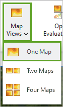
1. On the ribbon, on the Suitability Modeler tab, in the Views group, click the Map views button and choose One Map.

   

2. In the Contents pane, turn Gulf_Water back on. If necessary, zoom to the Nicoya_Suitability layer extent.

   You’ll create a clause to define mangrove areas as restricted locations.

3. In the Suitability Modeler pane, click the Settings tab and expand the Identify restricted locations section.

   

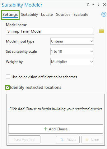
4. Click Add Clause, and form the clause Where Land_Cover Class_Name is equal to Mangrove.

   

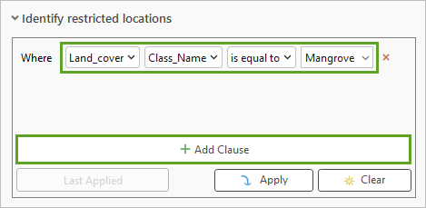
   Any area of the Land_Cover layer that is identified as Mangrove will become off limits.

5. Click Add Clause, and form the clause Or Where Land_Cover Class_Name is equal to Built Area.

   

   Any area of the Land_Cover layer that is identified as Mangrove or Built Area will become off limits.

6. Click Apply and Apply Restricted.

   

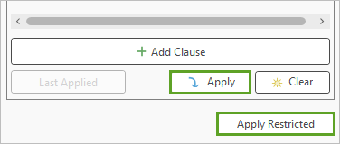
   On the map, a Restricted map layer now represents the mangrove and built areas in gray. These areas are no longer part of the combined suitability layer.

   

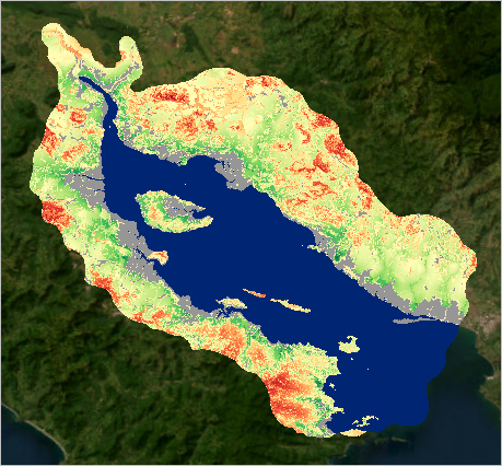
Weight model criteria relative to one another

You transformed the five criteria onto a common scale, and currently they all contribute equally to the combined suitability layer. However, you want to introduce more nuance, as some criteria may be more important than others when considering where to locate a shrimp farm. You will do that by assigning relative weights to the criteria.

For instance, it is critical that shrimp farms be located next to the gulf to ensure access to the briny water necessary for shrimp development. So, this criterion will receive the highest weight. In contrast, since the road network is good in most of the area of interest, the distance to roads criterion is not as essential, and it can receive a lower weight.

1. In the Suitability Modeler pane, in the Criteria table, review the Weight field.

   

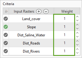
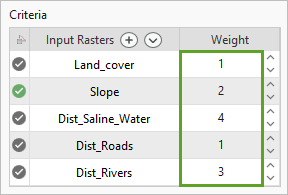
   Currently, all criteria are assigned a weight of 1, and as a result are equal in importance. Since the Dist_Saline_Water criterion is critical, you'll assign it a weight of 4. The Dist_Rivers criterion is next in importance, and you'll assign it a weight of 3. Slope will receive a weight of 2, and the remaining criteria a weight of 1.

2. In the Criteria table, update the Weight values as follows.

   Input Raster	Weight
   Land_Cover	1
   Slope	2
   Dist_Saline_Water	4
   Dist_Roads	1
   Dist_Rivers	3

3. Click anywhere in the pane to apply the weights. In the Criteria table, confirm your Weight values before continuing.

   

   Note:

   The order in which the criteria are listed may vary.

4. Review the resulting Nicoya_Suitability layer.

   

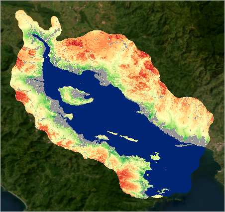
   This represents your final suitability map. Notice that areas located close to the gulf, rivers, and low slope areas are the most suitable (in green). Areas that are farther from these features are least suitable and symbolized in red.

   In the Contents pane, you can see that the suitability value range now goes up much higher, to 104.

   

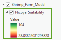
   This is because the weights are multipliers: each criterion's suitability value is multiplied by the criterion's weight. Since the maximum value is 10 for each criterion, the total maximum suitability based on the weights you chose is theoretically the following:

   10 * 4 + 10 * 3 + 10 * 2 + 10 * 1 + 10 * 1 = 110

   During the exploratory stage of the model creation, the Suitability Modeler was processing at screen resolution and extent, and the layers generated were only saved in memory. Before moving on to the next phase of your workflow, you must run the model at full resolution and save the Nicoya_Suitability layer to disk.

5. In the Suitability Modeler pane, at the bottom of the Suitability tab (under the Criteria table), click Run.

   

   When the process is complete, a green message indicates that it succeeded.

Locate the shrimp farms

You'll now use the Nicoya_Suitability layer to identify the five best locations for new shrimp farms. This is done in the Suitability Modeler on the Locate tab. The goal is to find regions that have the highest suitability possible, while also meeting a number of spatial requirements. For instance, spatial requirements can include the total area and number of regions desired, their minimum and maximum sizes, and the ideal distances between the regions.

1. In the Suitability Modeler pane, click the Locate tab.

   

   You'll consider the following spatial requirements for the shrimp farms.

   • Capacity and demand for the processing of shrimp at local plants is limited and therefore cannot service more than five new shrimp farms.
   • Each farm must be at least 3,000 hectares in size.
   • To avoid spreading diseases between farms, new farms must be sited at least 5 kilometers from one another.
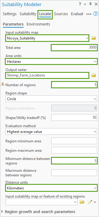
2. On the Locate tab, enter the following parameters:
   • For Input Suitability Map, confirm that Nicoya_Suitability is selected.
   • For Area units, select Hectares.
   • For Total area, type 3000 (this is best done after selecting the Area units).
   • For Output raster, type Shrimp_Farm_Locations.
   • For Number of regions, type 5.
   • For Minimum distance between regions, type 5.
   • For Distance units, confirm Kilometers is selected.
   • For all the other parameters, accept the default.

   

3. Click Run.

   The process may take a few moments.

   Note:

   The Locate tab calls the Locate Regions geoprocessing tool. To learn how the locate algorithm works, see How the Locate Regions tool works.

   The Shrimp_Farm_Locations layer appears.

4. Verify that five locations were identified.

   

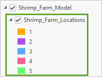
   Note:

   The colors are assigned at random and may vary.

5. To see the locations more clearly, in the Contents pane, turn on the Land_Mask layer. Ensure that only Shrimp_Farm_Locations and Restricted map display on top of it, and turn off any extraneous layers.
6. On the map, review the Shrimp_Farm_Locations layer and its five locations.

   

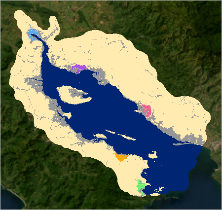
   The Land_Mask layer, displayed in cream color, shows the land that is part of the study area. The restricted mangrove and built areas still display in gray, and the proposed shrimp farm locations appear as spots of bright color.

7. Turn on the Nicoya_Suitability layer. On the map, pan and zoom to observe where the chosen regions are located compared to the suitability layer.

   

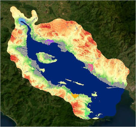
   All five regions are located in highly suitable areas (darker green). They also avoid mangrove areas completely.

8. Save the model.
9. Save the project.

Going further

Using the Suitability Modeler, you successfully identified the best locations in the Gulf of Nicoya for the development of five new sustainable organic shrimp farms. With the interactive, exploratory nature of the Suitability Modeler, you can continue your examination of the model using the tools on the Suitability Modeler tab to understand how the model components interact to produce the final results. You can create queries to examine how the base input criteria are realized in the final suitability map. For example, you can identify all locations that are within 1,000 meters of the gulf, are 500 meters from a river, and have received a suitability value greater than 100 on the final suitability map.

With the modeler, you can also explore what-if scenarios to see their impact. For example, what happens if a new treatment becomes available allowing you to locate the shrimp farms closer together? You can run the Suitability Modeler reducing the distance between the farms and see if you get different proposed locations. Moreover, you could explore adding other relevant criteria to the model, such as soil type or water salinity.

Apply this workflow to your own data - optional

Keep the following in mind if you want to prepare your own data to run a similar workflow on a study area of your choice.

Clipping layers:

• A vector layer can be clipped with the Clip or Pairwise Clip tools, and a raster layer with the Clip Raster tool.
• Use a vector layer, such as Study_Area, or a raster layer, such as Land_Mask, as the clipping extent.

Generating distance layers:

• The three distance layers used in this tutorial were generated using the Distance Accumulation tool (Spatial Analyst). For instance, to generate the Dist_Roads raster, the tool calculated the straight-line or Euclidean distance from each cell in the raster to the closest road, as represented in the Roads layer.
• In addition, there is only interest in computing these distance rasters for the land part of the study area (and not where the gulf water is located). For that reason, the Land_Mask layer was set as the analysis mask. This means that only the cells within the Land_Mask shape received a distance value.
• Finally, it is also important to use the same cell size for all distance rasters, for the purpose of the upcoming suitability analysis.
• Using the Roads layer as an example, this is how you would set the Distance Accumulation tool parameters:
  • For Input raster or feature source data, choose the Roads feature layer.
  • For Output distance accumulation raster, type Dist_Roads.
  • Leave the other parameters blank.
  • On the Environments tab, for Extent, Mask, and Snap raster, choose Land_Mask.
  • For Cell size, type 30 (meters).

Generating slope and hillshade layers:

• Starting from a terrain or digital elevation model (DEM) raster layer, use the Slope or Surface Parameters tools (Spatial Analyst) to generate the Slope layer.
• Starting from the same DEM layer, use the Hillshade tool (Spatial Analyst) to generate the Hillshade layer.

In this tutorial, you explored five criteria relevant for shrimp farming. You created a suitability model with the help of the Suitability Modeler, added the five criteria to it, transformed the criteria to a common 1-to-10 scale, defined restricted locations, weighted the criteria relative to each other, and located the five best locations for new shrimp farms. Because of the dynamic feedback you receive in the Suitability Modeler, you can be more confident of your input criteria, the model parameters, and final result obtained. The Suitability Modeler allows you to make informed decisions.

You can find more tutorials like this in the Introduction to Imagery and Remote Sensing tutorial collection.

Acknowledgements

• Roads feature class: Data downloaded from OpenStreetMap obtained from GeoFabrik.
• Rivers feature class: Data downloaded from OpenStreetMap obtained from GeoFabrik.
• Land_Cover raster: Derived from the ArcGIS Living Atlas Sentinel-2 10m Land Use/Land Cover Time Series (for 2023) and enriched with data from OpenStreetMap obtained from GeoFabrik.
• Slope and Hillshade rasters: Derived from the ArcGIS Living Atlas Terrain image service.
• Study_Area feature class: Created by the tutorial’s authors.
• All other data layers are derived from the layers listed above.
• World Imagery layer sources: Esri, Maxar, Earthstar Geographics, and the GIS User Community
• All Adobe Stock images are ©2025 Adobe Stock. All rights reserved.