Extract 3D buildings using photogrammetry

Today, there is a variety of technologies that are used to create 3D data for mapping houses, forests, and other natural or constructed features. A common process for creating such data is light detection and ranging (lidar). However, photogrammetry is another method of generating 3D data within GIS. Photogrammetry is the science of taking two images of the same object and obtaining reliable height and depth measurements to map the object's physical characteristics. When these images are collected as part of an aerial survey, photogrammetry allows you to map your entire community in 3D with precision.

In this tutorial, you'll take the existing building footprints for a local subdivision of Pleasanton, California, and turn them into 3D models with accurate heights and correctly shaped roofs. The city government requires each building to have attribution that records the building height and roof characteristics, so you'll also add this attribution. Not only is the 3D attribute information valuable for appraisers, it can be used for a variety of use cases across the government enterprise in emergency management, facility management, planning, and Building Information Modeling (BIM).

This tutorial was last tested on August 6, 2026, using ArcGIS Pro 3.7. If you're using a different version of ArcGIS Pro, you may encounter different functionality and results.

Requirements

• ArcGIS Pro Advanced (see options for software access)
• Publisher or Administrator role in an ArcGIS organization: ArcGIS Online (see options for software access) or ArcGIS Enterprise (learn more)

Access photogrammetry data

The City of Pleasanton's Appraisal Department has given you access to aerial imagery products from Nearmap and the building footprints for a subdivision at the base of Pleasanton Ridge. Once you have this data downloaded, you'll add it to an ArcGIS Pro project that is a part of the 3D Buildings solution. Together, they will lay the foundation for creating a 3D model of this community.

Acquire the data and project

First, you'll download and unzip the Nearmap data for Pleasanton. Then, you'll download an ArcGIS Pro project with steps to help build 3D models.

1. Download the Pleasanton.zip file. Extract the file to a suitable location on your computer.

   Next, you'll download a ArcGIS Pro project from ArcGIS Solutions, a collection of industry-specific apps, maps, and workflows. You'll use the 3D Buildings solution, which is configured for mapping 3D buildings.

2. Sign in to your ArcGIS organizational account.

   Note:

   If you don't have an organizational account, see options for software access.

3. On the ribbon, click the apps button and choose Solutions.

   

   A gallery of solutions appears.

4. In the search bar, type 3D Buildings.
5. In the list of results, click the 3D Buildings solution.

   

   A page appears with more information about the solution. According to the page, this solution can be used to develop a standard set of 3D layers and visualize a community in an immersive way.

6. Click Deploy.

   

   To deploy a solution, you have to give it a unique name.

7. In the Deploy 3D Buildings window, for Solution name, type 3D Buildings and add your name or initials to make the name unique. Click Deploy.

   The solution is deployed. You go to the page for your deployment, which lists the items included in it. The deployment contains one item, a desktop application template that can be opened in ArcGIS Pro.

8. Under Contents, expand Desktop Application Template (1). Click 3DBuildings.

   

   The 3DBuildings details page appears, listing more information about the item. You'll download the item so you can use it in ArcGIS Pro.

9. Click the Download button.

   

   A zipped folder named 3DBuildings is downloaded to your computer's default download location.

10. Extract the 3DBuildings .zip file to a suitable location on your computer.

    Note:

    Make sure that the file path to your 3DBuildings folder does not contain any files with spaces. Spaces in the file path will cause an error later in the workflow.

Add data to the project

Now that you have the required data from the city and the solution's ArcGIS Pro project, you'll add the city's data to the 3D Buildings solution's scene, or 3D map.

1. Open the 3DBuildings folder and double-click the 3DBuildings ArcGIS project file (.aprx) to open it in ArcGIS Pro. If prompted, sign in to your ArcGIS account.

   Note:

   If you don't have access to ArcGIS Pro or an ArcGIS organizational account, see options for software access.

   The project opens, showing a default 3D scene. You'll add the Pleasanton data to the scene.

2. On the ribbon, click the Map tab. In the Layer group, click the Add Data button.

   

   The Add Data window appears.

3. Browse to the location where you extracted the Pleasanton folder. Open the Pleasanton folder and the Pleasanton geodatabase.

   

   You'll add the AI_Buildings, DSM, and DTM datasets to the scene.

4. Press the Ctrl key and select the AI_Buildings, DSM, and DTM datasets. Click OK.

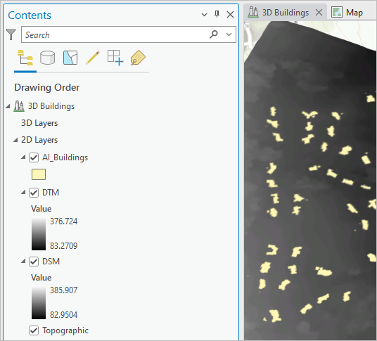
   The layers are added to the scene.

   

   Note:

   The buildings layer has random symbology. Its color may differ from the example image. The color of the layer will not affect the workflow.

   The AI_Buildings polygon layer represents building footprints derived from Nearmap's artificial intelligence and machine learning algorithms.

   The DSM raster layer is a digital surface model. Each pixel in this raster represents the elevation of the terrain as well as above-ground features such as buildings, vegetation, towers, and other infrastructure.

   The DTM raster layer is a digital terrain model. Also known as a digital elevation model (DEM), each pixel represents the elevation of the bare earth. It does not include the elevation of features on the landscape, such as trees or buildings.

   The DSM and DTM rasters have a resolution of 12 inches. In other words, each pixel represents an area on the earth that is 12 inches by 12 inches. When working with rasters, it is typically a best practice to use rasters that have the same resolution.

   Note:

   If you are a Nearmap subscriber and want to use your own data, use the Map Browser's Export 3D tool to extract the DSM and DTM for your area of interest. AI content is accessible via API and offline deliveries. To learn more about how to access Nearmap AI read Access AI Content.

   Next, you'll rename the AI_Buildings layer.

5. In the Contents pane, click the AI_Buildings layer to select it.
6. Press the F2 key. Type Building Footprints and press Enter.

   

7. On the Quick Access Toolbar, click the Save Project button.

   

Now that the data has been downloaded and added to the scene, you're ready to start processing the buildings.

Generate 3D buildings

The ArcGIS Pro project that you downloaded includes a series of tasks to help guide you through the process of taking your datasets and generating 3D models from them. You'll use your three layers and these tasks to create Pleasanton's 3D buildings. First, you'll create an nDSM, which will be necessary when you want to give your building footprints height and a properly shaped roof.

Create an nDSM

An nDSM (normalized digital surface model) is created when a DTM is subtracted from a DSM. The result is an elevation raster that represents the ground-level elevations of features, as well as their height. You'll use a raster function to create an nDSM.

1. On the ribbon, click the Imagery tab. In the Analysis group, click the Raster Functions button.

   

   The Raster Functions pane appears.

2. In the Raster Functions pane, expand Math and click Minus.

   

   The Minus raster function subtracts one raster dataset from another.

3. For Raster, choose DSM. For Raster2, choose DTM.

   

   Before running the function, you'll ensure that it processes with the correct pixel output type. This parameter determines the range of values that a particular raster file can store. You'll use 32 Bit Float to ensure that decimal places in your output raster are not lost.

4. Click the General tab.

   

5. For Output Pixel Type, choose 32 Bit Float.

   

6. At the bottom of the pane, click Create new layer.

   The Minus_DSM_DTM raster is added to the map.

   

7. Close the Raster Functions pane.
8. Rename the Minus_DSM_DTM layer to nDSM.

   You'll change the layer's symbology to better observe the data.

9. In the Contents pane, for nDSM, right-click the symbol. Click the drop-down menu and check the box next to Show names.

   

10. Click the drop-down menu and choose the Elevation #1 symbol.

    

    On the map, the layer symbology updates. To make this symbology clearer, you'll change the stretch type. The stretch type determines the histogram used when drawing a raster's colors on the map. Using the Histogram Equalize stretch type will better show elevation data in the scene.

11. On the ribbon, click the Raster Layer tab. In the Rendering group, click the Stretch Type drop-down menu and choose Histogram Equalize.

    

    The nDSM layer renders with the new stretch type. More detail is visible in the raster.

    

    With the nDSM created, you're ready to start working with the building footprints.

Process the building footprints

Next, you'll use a task included with the solution to clip the DSM raster to each building footprint. Then, you'll use the elevation to segment the roof. The result will be that each building footprint is subdivided based on which way the different parts of the roof are facing.

1. In the Catalog pane, expand Tasks and double-click 3D Buildings.

   Note:

   If you don't see the Catalog pane, on the ribbon, click the View tab. In the Windows group, click Catalog Pane.

   

   The Tasks pane appears. The 3D Buildings solution includes many tasks, but for the city's project, you'll focus on the Publish buildings task group.

   Note:

   If a window appears asking you to confirm a toolbox code to run, click Yes.

2. In the Tasks pane, expand Create and Publish 3D Buildings. Double-click Preprocess Building Footprints (optional).

   

   The first task step is Split building footprints using features. You won't use this step, so you'll skip it.

3. At the bottom of the pane, click Skip.

   

   You'll use the Segment building footprints using elevation task step. This step will give your building footprints a height and break them up based on their different roof sections.

4. For Building Footprints, choose Building Footprints. For Elevation Surface (DSM), choose DSM.

   

   Next, you'll set the spectral detail for the tool, or the level of importance given to height differences in your DSM. For example, in a downtown area with tall buildings that contain many roof facets at various heights, a lower spectral detail will result in segments created only where there are large changes in elevation. Conversely, row housing with smaller height differences between buildings may require a higher spectral detail to fully segment. Valid values range from 1.0 to 20.0. The default value is 13.

5. For Spectral Detail, ensure that the value is 13.

   Note:

   For this parameter, and those that follow, the default value is a good starting point. Depending on your own datasets, you may want to consider trying different values until you get your desired results.

   Next, you'll set the spatial detail, or the level of importance given to the proximity of features in your DSM. For example, to segment architecturally complex buildings with many smaller facets, you would want to use a higher spatial detail. To smooth over variations that do not need representation, such as air conditioning units or cars in a parking garage, you would use a lower spatial detail. Valid values range from 1.0 to 20.0. The default value is 13.

6. For Spatial Detail, ensure that the value is 13.

   Next, you'll set the minimum segment size. This parameter controls the minimum size of a potential segment in pixels. If a potential segment is less than the threshold set, the segment will be merged with a surrounding segment.

7. For Minimum Segment Size (In Pixels), ensure that the value is 555.

   

   Next, you'll set the regularization tolerance, or the maximum distance that segment polygons can be adjusted in the effort to regularize geometry to right angles and diagonals. With high-resolution surface rasters, it's a best practice to set a regularization tolerance that is 5 to 10 times the size of the pixels to smooth out any rigidness of the pixels while maintaining the detail of the high-resolution pixels.

8. For Regularization Tolerance, in the first parameter, type 2. Ensure that the second parameter is set to Meters.

   

9. For Output Segmented Buildings, delete the existing text and type Footprints.

   

   Note:

   When the tool is run, _segmented will be automatically added to the end of the output name.

10. Click Run.

    Note:

    The tool may make take several minutes to run depending on your computer's hardware.

    Now that the footprints have been processed, you can use them to create 3D structures.

11. Click Finish.

    

Create 3D buildings

Now that you have an nDSM and segmented building footprints, you're ready to make 3D models of the buildings. You'll use another task to aid this process.

Based on your input data, you'll create buildings with a level of detail 2 (LOD2). Level of detail refers to the geometric intricacy of your 3D models. There are four level of detail classifications that range from LOD0, which is less detailed, to LOD3, which is the most detailed:

• LOD0 is a flat polygon without height or segmentation characteristics.
• LOD1 is a 3D polygon containing height characteristics.
• LOD2 is a 3D polygon with roof shapes.
• LOD3 is a 3D polygon with roof shapes and details pertaining to the facade of the structure such as windows, doors, and so on.

One level of detail is not necessarily better than another, but you should always try to work with a level of detail that is appropriate for a project's need. For example, someone making a realistic street-level view of a city may want LOD3. For the City of Pleasanton's needs, LOD2 buildings are the appropriate amount of detail for assessing building height and classifying roof characteristics.

1. In the Tasks pane, double-click Create Buildings.

   

   The first step of this task, Extract roof form information, will determine the roof form of each building based on the datasets you created or obtained previously.

2. Input the following parameters:
   • For Buildings, choose Footprints_segmented.
   • For Elevation Surface (DSM), choose DSM.
   • For Ground Elevation Surface (DTM), choose DTM.
   • For Normalized Elevation Surface (nDSM), choose nDSM.
   • For Output Building Polygons, type Buildings_LOD2.

   

   Note:

   When the tool is run, _roofform will automatically be added to the end of the new dataset's name.

3. Expand RoofForm.

   

   The RoofForm parameters control when a roof is considered sloped or flat when each building is processed. You'll use the default values for these parameters.

4. Click Run.

   Note:

   The tool may take several minutes to run depending on your computer's hardware.

5. When the tool finishes running, click Next Step.

   

   The next step in the task appears. This step is to apply 3D symbology to the output buildings layer you just created. Some task steps involve running tools and others contain steps for you to follow on your own. In this case, you'll symbolize the buildings on your own.

   By default, 3D symbology was applied to the layer. However, the buildings have white facades and roofs, which doesn't emphasize the roof forms. You'll change the colors of the symbols.

6. At the bottom of the Tasks pane, click the Contents tab.

   

7. In the Contents pane, for the Buildings_LOD2_roofform layer, click the symbol.

   

   The Symbology pane appears with a gallery of symbols. You'll use a symbol from a rule package included in the solution.

8. In the Symbology pane, click the Properties tab.

   

9. Click the Layers button.

   

10. Scroll down to Display Options. For FacadeColor, choose Light Sienna.

    

    Tip:

    To see the name of a color in the color picker, point to it.

11. For RoofColor, choose Gray 50%.

    

12. At the bottom of the Symbology pane, click Apply.
13. Close the Symbology pane. In the Contents pane, rename the Buildings_LOD2_roofform layer to 3D Buildings.
14. Under 2D Layers, turn off every layer.

    

    You'll change the basemap to show satellite imagery as context for the 3D buildings.

15. On the ribbon, click the Map tab. In the Layer group, click Basemap and choose Imagery.

    

16. Tilt, pan, and zoom the scene to see the buildings in 3D.

    

    You'll also explore the attributes of the 3D buildings. The city requires detailed information about each building, not just its shape.

17. In the Contents pane, right-click 3D Buildings and choose Attribute Table.

    The layer's attribute table appears. The first few fields are from the original Building Footprints layer provided by Nearmap.

    

18. Scroll to the end of the table.

    

    Several fields were added when the LOD2 buildings were created. These fields contain all of the data that the city needs.

    • BLDGHEIGHT (Building Height) is the maximum height of the building.
    • EAVEHEIGHT (Eave Height) is the minimum height of the building. Buildings with no eave height have flat roofs.
    • ROOFFORM (Roof Form) is the shape of the roof. The roof form can be flat, gable, or hip.

    

    • BASEELEV (Base Elevation) is the base height of the building, usually equal to the ground elevation where the building is located.
    • ROOFDIR (Roof Direction) is the compass direction (in degrees) that the roof faces. Only gable roof forms have values for this field.
    • RoofDirAdjust (Roof Direction Adjusted) is the field that allows the adjustment of the roof direction. The default value is 0. A value of 1 will rotate the roof counterclockwise 90 degrees, while a value of 2 will rotate it 180 degrees. This field is used for manually editing roof forms that were incorrectly extracted.
19. Close the attribute table.
20. At the bottom of the Contents pane, click the Tasks tab. In the Tasks pane, click Finish.

Fuse buildings

Your 3D buildings are technically only a 2D polygon feature class with 3D symbology. To finalize your buildings, you'll make a 3D feature class. The process of converting data from 2D to 3D is known as fusing.

1. In the Tasks pane, double-click Fuse Buildings.

   

   This tool will take your 2D polygons with a 3D symbology and turn them into a multipatch feature class that stores your building data in 3D.

2. Set the following parameters:
   • For Building Layer, choose 3D Buildings.
   • For Unique ObjectID, choose BuildingFID.
   • For Output Building Multipatch, type Pleasanton_Buildings.

   

3. Click Finish.

   The tool runs and the task finishes. The Pleasonton_Buildings layer is added to the scene and the Contents pane.

4. Close the Tasks pane. In the Contents pane, turn off the 3D Buildings layer.

   There seems to be no change to the scene, because the Pleasanton_Buildings layer (which is still turned on) is identical to the 3D Buildings layer. This layer is saved as a multipatch feature class in the project geodatabase.

5. In the Catalog pane, expand Databases. Expand the 3DBuildings geodatabase.

   All of the datasets you created are in this geodatabase.

   Note:

   If any datasets are missing from the geodatabase, right-click the 3DBuildings geodatabase and choose Refresh.

   

   The symbol for Buildings_LOD2_roofform represents a 2D polygon feature class, while the symbol next to Pleasanton_Buildings represents a 3D multipatch feature class.

6. Save your project.

In this tutorial, you took a DSM, a DTM, and building footprints from Nearmap and converted them into a 3D model for the city to use for its planning and safety purposes. This workflow can be performed for any study area, as long as you have a DSM, DTM, and building footprints. Try creating a 3D multipatch feature class for your own city or area of interest.

You can find more tutorials in the tutorial gallery.

Acknowledgements

• The DSM, DTM, and building footprint datasets were all provided by Nearmap.
• The tutorial gallery image was obtained from Unsplash.
• World Imagery layer sources: Esri, Vantor, Earthstar Geographics, and the GIS User Community