Explore the data and map solar energy
You'll start by becoming familiar with the data and geography. Then, you'll create a raster layer that maps how much solar energy reaches rooftop surfaces in Glover Park over the course of a typical year. The more solar energy a roof surface receives, the more electric power could be generated if it were equipped with solar panels.
Open the project
First, you'll download a project that contains all the data for this tutorial and open it in ArcGIS Pro.
- Download the Solar_in_Glover zip file.
- Locate the downloaded file on your computer.
Note:
Most browsers download to your computer's Downloads folder by default.
- Right-click the file and extract it to a location you can easily find, such as a folder on your C: drive.
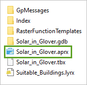
- Open the Solar_in_Glover folder, and double-click Solar_in_Glover.aprx to open the project in ArcGIS Pro.
- If prompted, sign in with your ArcGIS account.
Note:
If you don't have access to ArcGIS Pro or an ArcGIS organizational account, see options for software access.
The project opens.
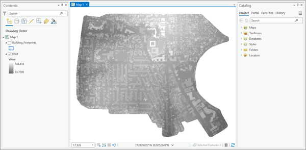
The project contains two layers: the DSM and Building_Footprints layers. You'll first explore the DSM layer.
The DSM layer, which is turned on by default, represents the neighborhood of Glover Park as a digital surface model (DSM). A DSM shows the elevation of the ground and the features on the ground, such as buildings and trees. This DSM is a raster layer, which depicts data in a grid in which each cell contains a numeric value. It is symbolized so that darker cells have lower elevations and lighter cells have higher ones.
- With the mouse wheel button, zoom in until you see the individual cells that compose the DSM raster.

In this raster, each cell represents a surface of 0.5 by 0.5 meters (about 1.6 by 1.6 feet).
- Click any cell.
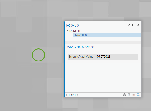
A pop-up window appears. It contains a value that represents the elevation (in meters) of the selected raster cell. In the example, the highlighted cell has an elevation of about 96.6 meters (or 316 feet).
- Close the pop-up.
- In the Contents pane, right-click DSM and choose Zoom To Layer.
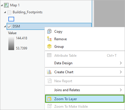
The map navigates back to the full extent of the Glover Park neighborhood.
Create a hillshade effect
Although patterns in the DSM suggest the locations of buildings and vegetation, you can better visualize the surface by creating a hillshade effect. A hillshade raster layer uses a realistic shading effect to depict elevation. You will create one with the Hillshade raster function.
- On the ribbon, click the Imagery tab. In the Analysis group, click the Raster Functions button.
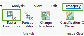
The Raster Functions pane appears.
Note:
Raster functions are tools that apply calculations directly to a raster's pixel values without requiring new data to be saved. As such, they are very efficient.
- In the Raster Functions pane search box, type hillshade. In the list of results, under Surface, click Hillshade.
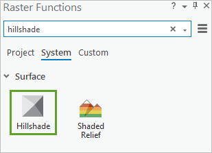
The Hillshade tool appears.
- For Raster, choose DSM. Accept all the other default values and click Create new layer.
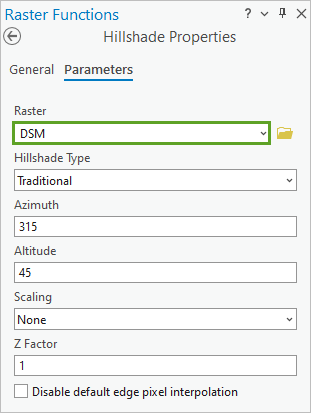
A new layer, named Hillshade_DSM, is added to the map. For optimum visual effect, you'll combine hillshade and DSM layer symbolization.
- In the Contents pane, drag the DSM layer above the Hillshade_DSM layer.
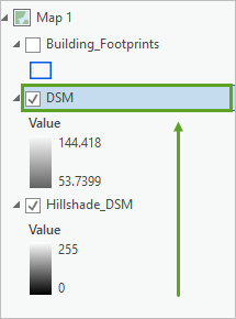
The DSM layer is set to 40 percent layer transparency. When it is drawn above the hillshade, both layers are visible.
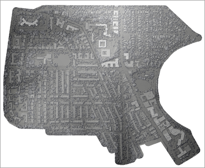
- Zoom in with the mouse wheel button until you can see the details of the landscape.
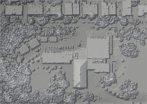
The hillshade layer's realistic shading added a 3D effect. Buildings, trees, and other surface features are more distinguishable. You can also distinguish whether buildings have flat or gabled (sloped) roofs, which is important for rooftop solar panels.
Note:
While you can symbolize the DSM layer with a more colorful color ramp, you'll keep the gray tones. Subdued tones form a good background that will allow the other layers you'll produce in this tutorial to be the center of attention.
- In the Contents pane, right-click DSM and choose Zoom to Layer to return to the full extent of the neighborhood.
Note:
The hillshade layer that you created with a raster function is computed dynamically and not written on disk. So, if you remove it from the Contents pane, it will disappear, and you'll have to re-create it.
Explore building footprints
The project contains a layer called Building_Footprints that is turned off by default. Next, you will explore this layer.
- In the Contents pane, check the box next to the Building_Footprints layer to turn it on.
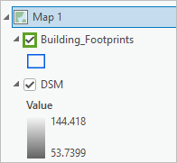
The layer contains outlines of every building in the Glover Park neighborhood. Unlike the DSM and hillshade layers, which are rasters, this is a vector layer, which displays spatial information in the form of polygons.
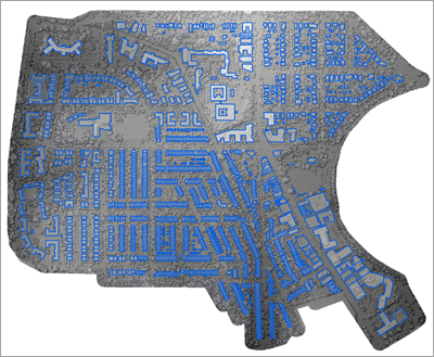
- Zoom and pan throughout the map to explore the neighborhood.
You can see that the neighborhood contains many types of buildings, from small single-family units to large commercial structures, as well as medium-sized multifamily units. Many areas also present a significant level of tree coverage, which can have an impact on solar power production.
- Return to the full extent of the neighborhood.
- On the Quick Access Toolbar, click the Save Project button to save the project.

Note:
A message may appear warning you that saving this project file with the current ArcGIS Pro version will prevent you from opening it again in an earlier version. If you see this message, click Yes to proceed.
Create a solar radiation layer
To create the solar radiation layer, you'll use the Raster Solar Radiation tool. This tool is part of the ArcGIS Spatial Analyst extension and takes a DSM as input. It calculates radiation based on a sophisticated model that takes into account the position of the sun throughout the year and at different times of day, obstacles that may block sunlight such as nearby trees or buildings, and the slope and orientation of the surface. You can read more about modeling solar radiation on the Modeling solar radiation, Analyze solar radiation, and How Raster Solar Radiation works documentation pages.
The DSM provides the necessary information on obstacles, orientation, and slope. The output will be a raster layer in which each cell value is the amount of solar radiation in kilowatt-hours per square meter (kWh/m2) at that location.
- On the ribbon, on the Analysis tab, in the Geoprocessing group, click Tools.
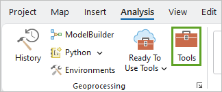
The Geoprocessing pane appears.
- Search for and open the Raster Solar Radiation tool.
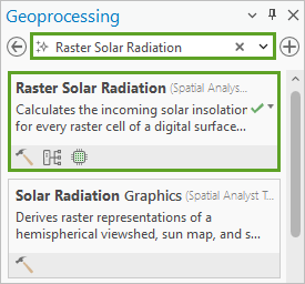
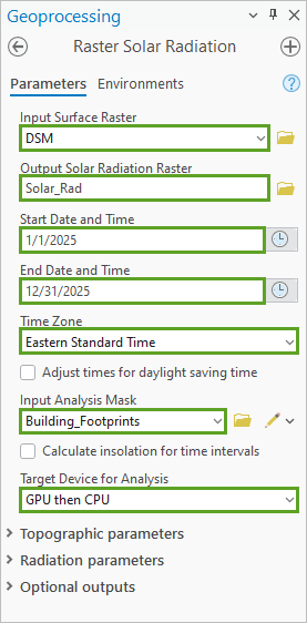
- Set the following tool parameters:
- For Input Surface Raster, choose DSM.
- For Output Solar Radiation Raster, type Solar_Rad.
- For Start Date and Time, click the calendar button, choose 1/1/2025, and click Date.
- For End Date and Time, click the calendar button, choose 12/31/2025, and click Date.
- For Time Zone, choose Eastern Standard Time.
- For Input Analysis Mask, choose Building_Footprints.
- For Target Device for Analysis, confirm that GPU then CPU is selected.
The tool will compute the total amount of solar radiation for the year 2025 for every pixel located within the building layer's polygons. Eastern Standard Time corresponds to the time zone for Washington, D.C. Finally, the tool will use your computer's GPU if there is one, and the CPU otherwise.
Note:
Learn more about GPU processing with Spatial Analyst.
- Click Run.
After a few minutes, the solar radiation layer appears.
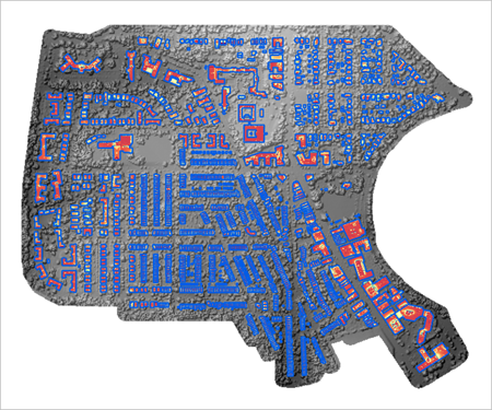
You won't need the Building_Footprints layer for the next steps, so you'll turn it off.
- In the Contents pane, uncheck Building_Footprints to turn it off.
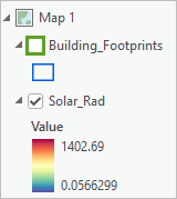
- Zoom in to better see the rooftop surfaces.
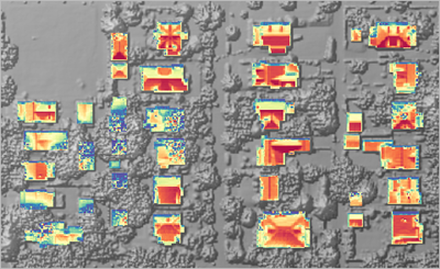
Red and orange colors indicate higher amounts of solar radiation, while yellow and blue tones indicate lower amounts. (The cells that are outside the Building_Footprints polygons have not been computed. They have a value of NoData and are not displayed.)
North-facing roof slopes have blue and yellow tones, as they tend to receive less solar energy than south-facing ones. Additionally, roofs blocked by trees or other buildings sometimes receive very little solar energy.
- Return to the full extent of the neighborhood.
- Press Ctrl+S to save the project.
In this module, you downloaded, opened, and explored the initial data for the project, which includes elevation data and building footprints. You also created a hillshade layer to better visualize the Glover Park neighborhood's surfaces. You then created a solar radiation raster layer to map the annual solar energy received on the neighborhood's rooftops. Next, you'll identify rooftops suitable for solar panels.
Identify suitable rooftops
To identify suitable rooftops for solar panels, you will consider three criteria:
- Suitable rooftops should have a slope of 45 degrees or less, as it is difficult to install solar panels on a steep roof. To determine rooftop slope, you must create a slope raster layer.
- Suitable rooftops should receive at least 800 kWh/m2 of solar radiation. You can assess this criterion using your solar radiation raster layer.
- Suitable rooftops should not face north, as north-facing rooftops in the northern hemisphere receive less sunlight. To determine rooftop orientation, you must create an aspect raster layer.
Create a slope layer
First, you will use the Surface Parameters tool to create a slope raster layer based on your DSM.
- In the Geoprocessing pane, click the Back button.

- Search for and open the Surface Parameters (Spatial Analyst Tools) tool.
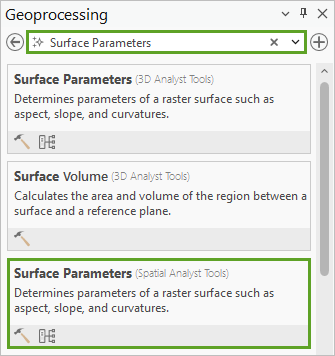
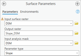
- Set the following tool parameters:
- For Input surface raster, choose DSM.
- For Output raster, type Slope_DSM.
- For Input analysis mask, confirm that DSM is selected.
- For Parameter type, confirm that Slope is selected.
The other parameters, which determine how a slope is measured and calculated, do not need to be changed.
- Click Run.
The tool runs and the new raster layer is added to the map.
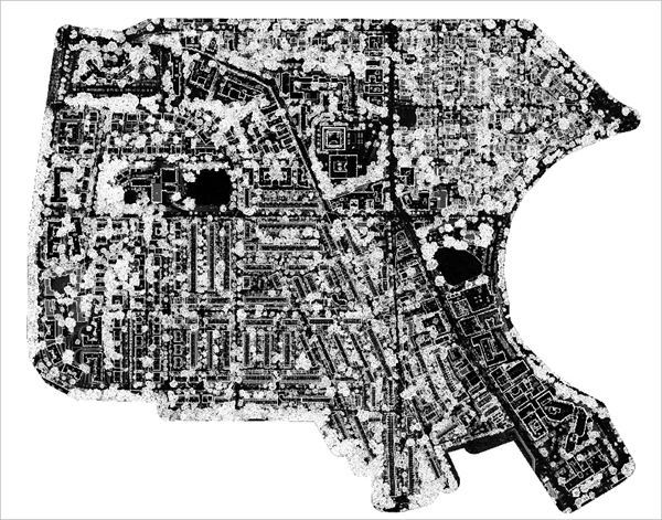
Each cell in this layer contains a slope value ranging from 0 to 90 degrees. The yellow and lighter green tones represent steeper slopes while the purple and dark blue tones represent the milder slopes.
Create an aspect layer
To determine the rooftop orientation, you will create an aspect raster layer using the Surface Parameters tool.
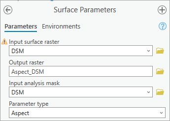
- In the Surface Parameters tool pane, set the following parameters:
- For Input surface raster, keep DSM.
- For Output raster, type Aspect_DSM.
- For Input analysis mask, keep DSM.
- For Parameter type, choose Aspect.
You do not need to change the method by which the tool will calculate aspect.
- Click Run.
The tool runs and the new raster is added to the map.
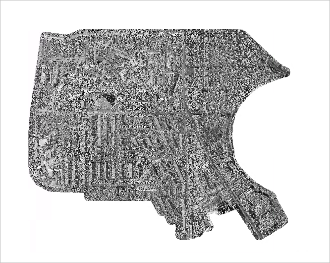
Each cell contains a value expressing orientation in degrees, with 0, 90, 180, and 270 representing absolute north, east, south, and west, respectively.
Note:
It is possible to generate the slope and aspect layers earlier in the workflow, and use them as optional input in the Raster Solar Radiation tool (under Topographic parameters). This will improve the performance, as the tool won't need to compute the slope and aspect values on the fly. This is particularly useful if you are working with a large extent.
Remove areas with high slopes
Next, you will use your raster layers to find areas that meet the criteria for solar panels. First, you'll remove areas from your solar radiation raster layer that have a slope steeper than 45 degrees.
All of your raster layers use the same cell grid. Because of this, you can compare the values in the solar radiation and slope layers. You will create an expression in the Con tool that checks whether each slope value is less than or equal to 45. If a cell's slope is steeper than 45 degrees, its value will be changed to NoData in the output layer. Otherwise, the cell will be given its corresponding solar radiation value. The result will be a solar radiation raster layer that does not include slopes steeper than 45 degrees.
- In the Geoprocessing pane, click the Back button.
- Search for and open the Con tool.
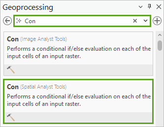
- In the Con tool pane,
for Input conditional raster, choose Slope_DSM. Under Expression, build the expression Where VALUE is less than or equal to 45.
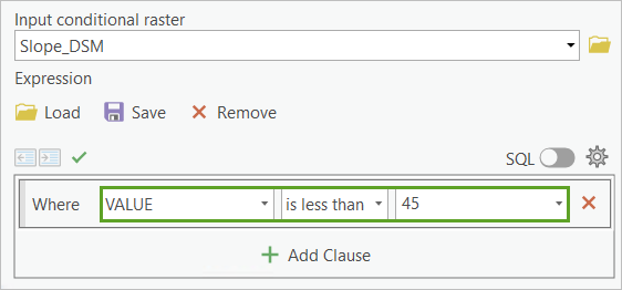
This expression will be applied to every cell in the slope raster. If a cell has a value less than or equal to 45, that cell is considered true. If not, the cell is considered false.
Next, you will choose the raster layer that will provide the output cell values for cells found to be true. Ultimately, you want to compute the solar radiation potential of the rooftops, so you'll have the output layer use solar radiation cell values.
- For Input true raster or constant value, choose Solar_Rad.
For the cell values found to be false, you have the option to choose a raster layer or set a constant value. However, you'll leave this parameter empty so that false cells are given the NoData value.
- For Output raster, change the output name to Solar_Rad_S (S stands for slope).
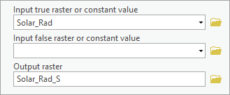
- Click Run.
The new raster is added to the map. Before you explore the new layer, you'll turn off some other layers to simplify your map view.
- In the Contents pane, uncheck the boxes next to Aspect_DSM and Slope_DSM to turn these layers off.
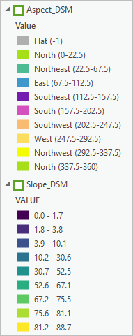
To make some space in the Contents pane, you'll also collapse the legends for these layers.
- Click the arrows next to Aspect_DSM and Slope_DSM to collapse them.
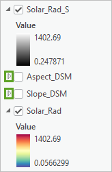
Next, you'll change the symbology of the Solar_Rad_S layer to match the Solar_Rad layer.
- In the Contents pane,
click the Solar_Rad_S color ramp to open the Symbology pane.
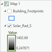
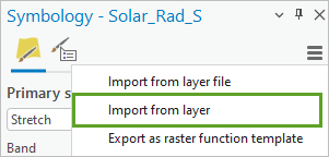
- In the Symbology pane, click the options button and choose Import from layer.
- In the Apply Symbology From Layer tool pane, for Input Layer, confirm that Solar_Rad_S is selected, for Symbology Layer, choose Solar_Rad, and click Run.
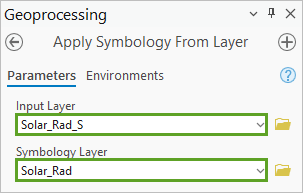
The Solar_Rad_S layer updates to the new symbology. You'll now use the Swipe tool to compare the two layers.
- Close the Symbology pane.
- In the Contents pane, confirm that the Solar_Rad and Solar_Rad_S layers are turned on. Click Solar_Rad to select it.
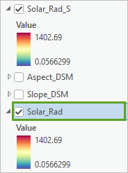
- On the ribbon, on the Raster Layer tab, in the Compare group, click Swipe.
- Zoom in with the mouse wheel to view some of the buildings in more detail.
- Drag the Swipe pointer from top to bottom to peel off the Solar_Rad layer and see what areas have been removed in the Solar_Rad_S layer.
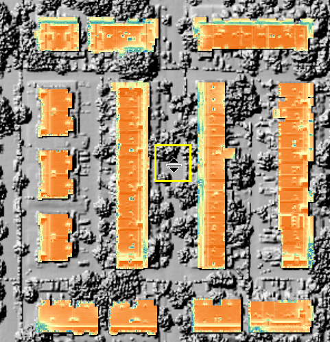
The removed areas are the rooftops with slopes above 45 degrees.
Note:
While swiping, to explore more areas, you can zoom in and out with the mouse wheel button. To pan, you can press the C key while dragging.
- Return to the full extent of the neighborhood.
- Press Ctrl+S to save the project.
Remove areas with low solar radiation
Next, you will consider the second criterion for suitable rooftops. Rooftop surfaces should receive at least 800 kWh/m2 in solar radiation, if solar panels are to be installed. You'll use the Con tool on the Solar_Rad_S layer to remove any remaining areas with low solar radiation.
You'll open the History pane to easily access the Con tool.
- On the ribbon, on the Analysis tab, in the Geoprocessing group, click History.
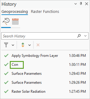
The History pane lists all the tools you have used so far.
- In the History pane, double-click Con to reopen the tool.
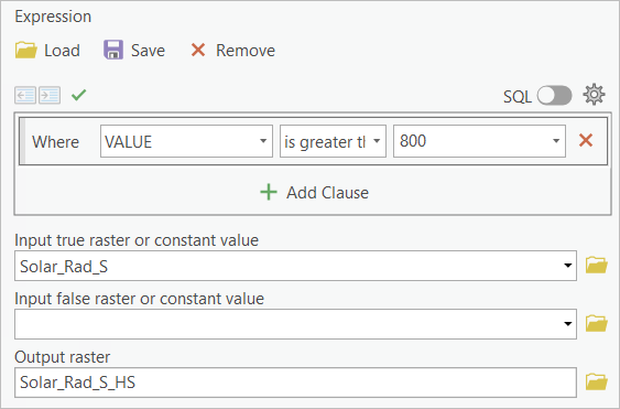
- In the Con tool pane, set the following parameters:
- For Input conditional raster, choose Solar_Rad_S.
- Under Expression, change the expression to read Where VALUE is greater than or equal to 800.
- For Input true raster or constant value, choose Solar_Rad_S.
- For Output raster, change the output name to Solar_Rad_S_HS (HS stands for high solar).
- Click Run.
The new raster layer is added to the map. You'll symbolize it the same way you symbolized the other solar radiation layers.
- At the bottom of the Geoprocessing pane, click the History tab to return to that pane.

- In the History pane, double-click Apply Symbology From Layer.
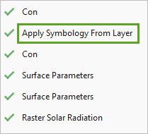
- In the Apply Symbology From Layer tool pane, for Input Layer, choose Solar_Rad_S_HS, and for Symbology Layer, confirm that Solar_Rad is selected. Click Run.
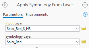
The symbology is applied to the layer.
- In the Contents pane, turn off the Solar_Rad layer. Click the Solar_Rad_S layer to select it.
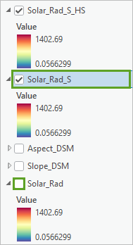
- If necessary, on the ribbon, on the Raster Layer tab, click Swipe.
Note:
The Swipe tool should still be on from your earlier use.
- With the Swipe tool,
inspect how the Solar_Rad_S and Solar_Rad_S_HS layers differ.
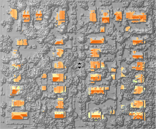
More unsuitable areas have been removed. These areas received low solar radiation, making them undesirable for solar panels.
- Return to the full extent of the neighborhood.
- Press Ctrl+S to save the project.
Remove areas that face north
The third criterion for suitable rooftops is that roof surfaces should not face north. In the northern hemisphere, surfaces facing north are likely to receive less solar radiation than surfaces facing other directions. (In the southern hemisphere, south-facing surfaces receive the least solar radiation.)
Many north-facing roof surfaces were already eliminated when you removed areas with low solar radiation, but some remain. Based on the Aspect_DSM legend, slopes that face north have a value less than 22.5 degrees or more than 337.5 degrees. This means that you want to keep only slopes with a value more than 22.5 degrees and less than 337.5 degrees. Additionally, you want to keep slopes that are almost flat, regardless of their aspect. If a roof is almost flat, it doesn't matter if it is facing north or not. You will consider that slopes of 10 degrees or less are flat or almost flat.
To fulfill both conditions, you'll use both Aspect_DSM and Slope_DSM. You'll run the Con tool twice, first to determine areas with low slopes and then to determine areas that don't face north.
- Switch to the History pane and double-click Con (either of the two instances).
- In the Con tool pane, set the following parameters:
- For Input conditional raster, choose Slope_DSM.
- Form the expression Where VALUE is less than or equal to 10.
- For Input true raster or constant value, choose Solar_Rad_S_HS.
- For Output raster, change the output name to Solar_Rad_Low_Slope.
- Click Run.
The new raster layer is added to the map, it contains only surfaces with low slopes. You will now run the Con tool a second time to determine surfaces that aren't north facing. These are slopes that have a value more than 22.5 and less than 337.5. Your expression will require two clauses to fulfill both of these conditions. You will also use the Input false raster parameter to ensure that you keep north facing surfaces if they are low slope.
- In the Con tool pane, set the following parameters:
- For Input conditional raster, choose Aspect_DSM.
- Form the expression Where VALUE is greater than 22.5.
- Click Add Clause and create the second expression And VALUE is less than 337.5.
- For Input true raster or constant value, confirm that Solar_Rad_S_HS is selected.
- For Input false raster or constant value, choose Solar_Rad_Low_Slope.
- For Output raster, type Solar_Rad_S_HS_NN (NN stands for no north).
As before, you are using Solar_Rad_S_HS as the true raster, and this time the conditional clauses ensure that only the non-north facing surfaces are kept. You are also adding the Solar_Rad_Low_Slope layer as the false raster, with the result that false cells (those that face north) will be replaced by values from the low slope layer. This means that the output layer will contain surfaces that don't face north, but also low slope surfaces (even if they face north).
- Click Run.
The new raster layer is added to the map. You will symbolize it the same way you have symbolized the other solar radiation layers.
- Switch to the History pane, and double-click Apply Symbology From Layer.
- In the Apply Symbology From Layer tool pane, for Input Layer, choose Solar_Rad_S_HS_NN, and for Symbology Layer, confirm that Solar_Rad is selected, and click Run.
- In the Contents pane, turn off the Solar_Rad_Low_Slope and Solar_Rad_S layers. Select the Solar_Rad_S_HS layer.
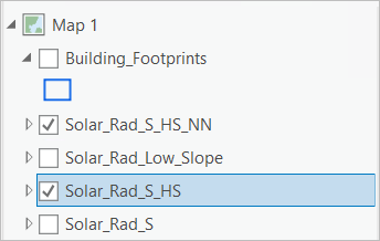
- With the Swipe tool,
inspect how the Solar_Rad_S_HS and Solar_Rad_S_HS_NN layers differ.
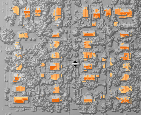
Because many north-facing surfaces were removed previously when you removed areas with low solar radiation, the change between these layers is not so dramatic. However, some areas did get removed, and the Solar_Rad_S_HS_NN layer contains only roof surfaces suitable for solar panels.
Note:
For actual solar panel installation, it would be necessary to look at each rooftop in more detail, but for the purpose of your analysis, this approximation is sufficient.
- When you are done exploring, on the ribbon, on the Map tab, in the Navigate group, click Explore to deactivate the Swipe tool.
- In the Contents pane, turn off Solar_Rad_S_HS.
For clarity, you'll rename the Solar_Rad_S_HS_NN layer.
- In the Contents pane, click Solar_Rad_S_HS_NN once to select it and a second time to enter edit mode, type Suitable_Cells, and press Enter.
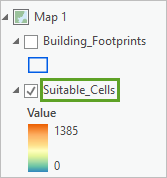
- Return to the full extent of the neighborhood.
- Press Ctrl+S to save the project.
In this module, you started from the initial solar radiation raster and removed all areas that are unsuitable for solar panels. You now have a suitable surface raster that you'll use to continue your analysis.
Calculate power per building
Your map shows how much solar radiation each suitable raster cell receives. In this module, you'll aggregate that data to determine how much solar radiation each building receives in a typical year. Then, you'll convert the solar radiation to electric power production potential and examine the results.
Aggregate cells by building
First, for every building, you'll calculate the area covered by its suitable cells (in m2) and their average solar radiation (in kWh/m2). You'll do that using the Zonal Statistics as Table tool.
- In the Contents pane, turn off the DSM and Hillshade_DSM layers. Turn on the Building_Footprints layer.
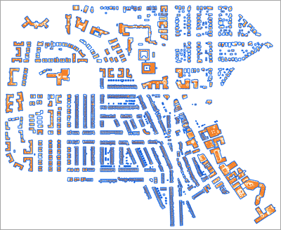
The Zonal Statistics as Table tool will look within each building footprint polygon and aggregate the suitable cells it contains.
- If necessary, on the ribbon, on the Analysis tab, click Tools to open the Geoprocessing pane. If necessary, in the Geoprocessing pane, click the Back button.
- Search for and open the Zonal Statistics as Table tool.
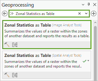
- In the Zonal Statistics as Table tool pane, set the following parameter values:
- For Input Raster or Feature Zone Data, choose Building_Footprints.
- For Zone Field, confirm that Building_ID is selected.
- For Input Value Raster, choose Suitable_Cells.
- For Output Table, type Solar_Rad_Table.
- For Statistics Type, choose Mean.
The Building_ID field is a unique identifier for each building footprint. Using this field as the zone field will ensure that each building footprint is clearly identified.
You can calculate several types of statistics. You'll calculate the Mean to determine the average solar radiation per square meter for each building.
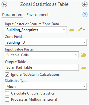
- Click Run.
The tool runs and the new table is added to the bottom of the Contents pane, under Standalone Tables.
Tip:
Your Contents pane contains many layers, so you may need to scroll down to see the table.
- In the Contents pane, right-click Solar_Rad_Table and choose Open.
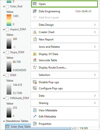
The table opens.
- Review the content of the table.
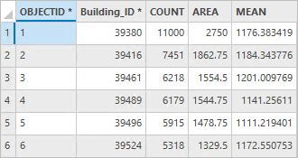
- Each row represents a building, uniquely identified by its Building_ID.
- COUNT gives the number of suitable cells for that building.
- AREA gives the area covered by suitable cells (in m2).
- MEAN gives the average solar radiation (in kWh/m2) that these cells receive.
Because this table is stand-alone, it is not connected to the spatial data on your map. You'll join the fields of interest, AREA and MEAN, to the Building_Footprints layer using the Join Field tool. The matching field for this join will be Building_ID.
- Close the table.
- In the Geoprocessing pane, click the Back button. Search for and open Join Field.
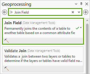
- In the Join Field tool pane, set the following values:
- For Input Table, choose Building_Footprints.
- For Input Field, choose Building_ID.
- For Join Table, choose Solar_Rad_Table.
- For Join Field, choose Building_ID.
- For Transfer Fields, choose AREA.
- For the second Transfer Fields drop-down list that appears, choose MEAN.
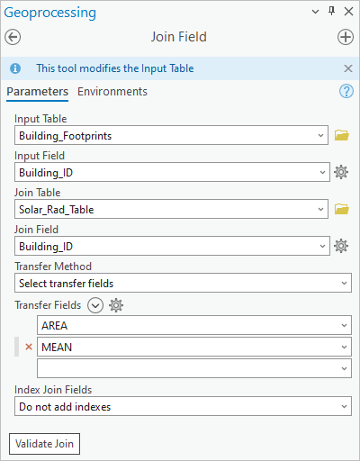
- Click Run.
After a few moments, the process completes.
- In the Contents pane, right-click Building_Footprints and choose Attribute Table.
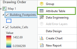
The AREA and MEAN fields have been added to the end of the table.

- Close the table.
Find suitable buildings
Now that you know the size of the suitable area on each building rooftop, you will apply one last criterion to determine solar panel suitability. You will consider that if a building has less than 30 square meters of suitable roof surface, it is generally not suitable for solar panel installation, as it is not worth the installation investment. You'll select buildings that have enough suitable roof surface using the Select Layer By Attribute tool.
- On the ribbon, on the Map tab, in the Selection group, click Select By Attributes.

- In the Select By Attributes window, set the following parameters:
- For Input Rows, confirm that Building_Footprints is chosen.
- For Selection type, confirm that New selection is chosen.
- Under Expression, create the expression Where AREA is greater than or equal to 30.
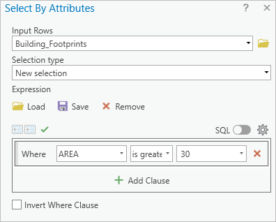
- Click OK.
The selection is applied. Many buildings are selected (in cyan color) but some are not.
- At the bottom of the map, view the exact Selected Features number.

Note:
Your number of buildings selected may be slightly different than in the example image.
- Zoom in to view some of the buildings in more detail.
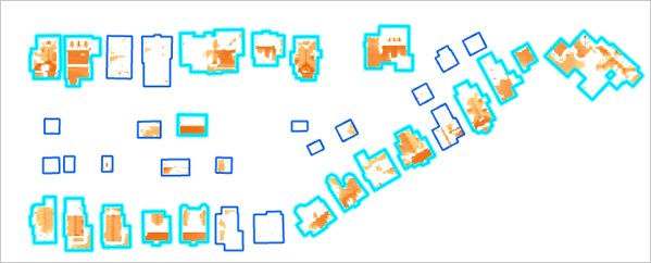
Many buildings that were not selected are particularly small, such as garden sheds. Others are larger but lack suitable surfaces for solar panels, possibly due to the shade produced by nearby trees or other buildings.
- Close the Building Footprints attribute table and return to the full extent of the neighborhood.
You'll export the selected buildings into a new feature class.
- In the Contents pane, right-click Building_Footprints, point to Data, and choose Export Features.
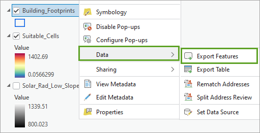
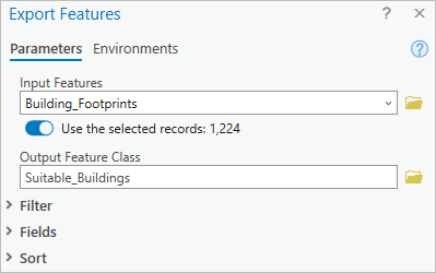
- In the Export Features window, for Input Features, confirm that Building_Footprints is selected. For Output Feature Class, type Suitable_Buildings.
Note:
The Use the selected records option is on, which ensures that only the buildings currently selected will be copied to the new layer.
- Click OK.
The new layer is created and added to the map.
- In the Contents pane, turn off the original Building_Footprints layer.
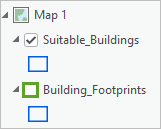
You now have a map of all the suitable buildings, and for each building, the suitable area they contain and their mean solar radiation per square meter.
Create a field for solar radiation
Next, you'll create a field in the Suitable_Buildings attribute table. This field will contain the total amount of solar radiation received per year by each building's usable area. You'll calculate this field by multiplying each building's suitable area by its average solar radiation per square meter. To avoid the numbers becoming too large, you'll also convert the solar radiation from kilowatt-hours to megawatt-hours by dividing by 1,000. The corresponding formula will be: (Area * Mean) / 1000.
- In the Contents pane, right-click Suitable_Buildings and choose Attribute Table.
- On the ribbon of the attribute table, click the Add Field button.
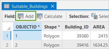
The Fields view appears. In this view, you can edit existing fields or add new ones.
- On the bottom row of the Fields view, for Field Name, type Usable_SR_MWh. For Data Type, double-click the cell and choose Double.
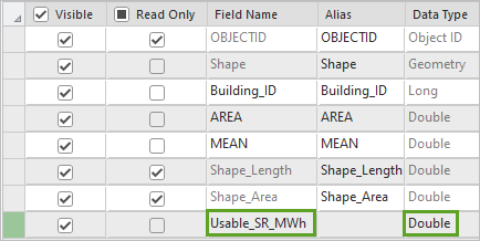
Note:
The Double data type is meant to store decimal numbers.
You'll have the field round all values to 2 decimal places.
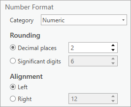
- For Number Format, double-click the empty cell and click the Determine display formatting for numeric and data field types button.

The Number Format window appears.
- In the Number Format window, for Category, choose Numeric. Under Rounding, for Decimal places, type 2.
- Click OK.
- On the ribbon, on the Fields tab, in the Manage Edits group, click Save.

The field is saved and added to the attribute table.
- Click the Suitable_Buildings tab to go back to the attribute table.

Currently, the values of the new field, Usable_SR_MWh, are all null.
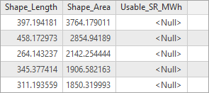
You'll calculate values for the field based on the values in the AREA and MEAN fields.
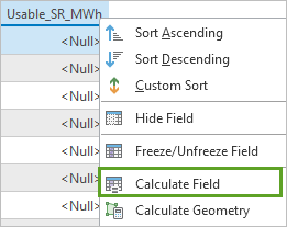
- In the attribute table, right-click the Usable_SR_MWh column name and choose Calculate Field.
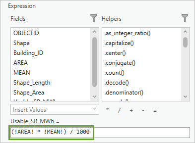
In the Calculate Field tool, you'll create an expression with the formula delineated above.
- In the Calculate Field window, under Usable_SR_MWh =, type or copy the following expression:
(!AREA! * !MEAN!) / 1000
- Click OK.
The tool runs and the field is populated.
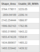
The results are expressed in megawatt-hours.
You now have an estimate of how much solar radiation every building receives each year on surfaces suitable for solar panels.
Convert solar radiation to power
Next, you will convert the usable solar radiation values to electric power production potential. The amount of power that solar panels can produce depends not only on solar radiation, but also the solar panels' efficiency and the installation's performance ratio.
You'll use the values of 21.6 percent efficiency and 83 percent performance ratio. This means that the solar panels are capable of converting 21.6 percent of incoming solar energy into electricity, and then 83 percent of that electricity is preserved as it goes through the installation.
Note:
Efficiency and performance ratios are not fixed numbers. Overall, they are improving over time as the photovoltaic technology advances, moreover, they also vary based on the specific solar panel type and installation conditions. The values chosen in this tutorial come from a 2024 report written by the Fraunhofer Institute for Solar Energy Systems, a prominent research center in the field of photovoltaic and solar energy technologies. According to the report, the current average efficiency for crystalline silicon photovoltaic units—the predominant solar panel type—is 21.6 percent (page 33), and the current typical performance ratio is 83 percent (page 34).
If you decide to apply this workflow to your own area of interest, you might choose slightly different values based on your knowledge of the local situation.
To determine the electric power production potential, you'll create a field and calculate it by multiplying your usable solar radiation values by the efficiency and performance ratio values. The corresponding formula will be: Usable_SR_MWh * 0.216 * 0.83.
- Click the Fields: Suitable_Buildings tab to switch back to the Fields view.

- In the Fields view, click Click here to add a new field.
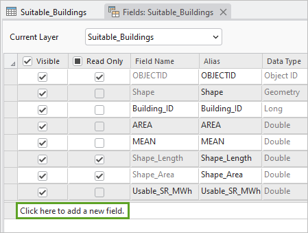
- For the Field Name text box, type Elec_Prod_MWh. For Data Type, choose Double.
- For Number Format, double-click the empty cell and click the Determine display formatting for numeric and data field types button.
- In the Number Format window, for Category, choose Numeric. Under Rounding, for Decimal places, type 2. Click OK.
- On the ribbon, on the Fields tab, in the Manage Edits group, click Save.
- Click the Suitable_Buildings tab to switch back to the attribute table.
The new field is added to the attribute table. Its values are null. Next, you'll calculate the field values.
- In the attribute table, right-click the Elec_Prod_MWh column name and choose Calculate Field.
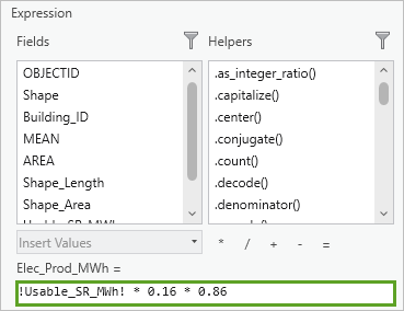
- In the Calculate Field window, under Elec_Prod_MWh =, create or copy and paste the following expression:
!Usable_SR_MWh! * 0.216 * 0.83
- Click OK.
The tool runs and the field is populated.
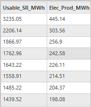
- Close the attribute table and the Fields view.
Symbolize the data
Your analysis is complete. Before you explore the results, you'll symbolize the layer based on the field you created—you'll apply a layer file with a predefined symbology that was included with the project data you downloaded. You will also add a basemap for context.
- Switch to the History pane, and double-click Apply Symbology From Layer.
- In the Apply Symbology From Layer tool pane, for Input Layer, choose Suitable_Buildings. For Symbology Layer, click the Browse button.

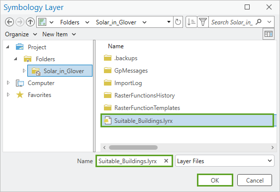
- In the Symbology Layer window, browse to the Solar_in_Glover folder, select Suitable_Buildings.lyrx, and click OK.
- Leave the other parameters unchanged and click Run.
The layer symbology updates.
- In the Contents pane, turn off all the layers except Suitable_Buildings.
Tip:
To turn off all layers, hold Ctrl and click one of the layer boxes.
- On the ribbon, on the Map tab, in the Layer group, click Basemap. Choose Dark Gray Canvas.
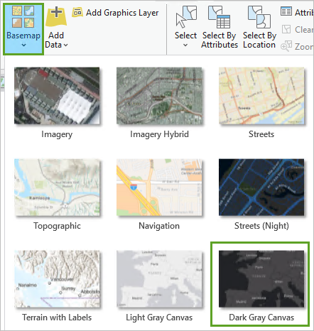
The basemap is added to the map.
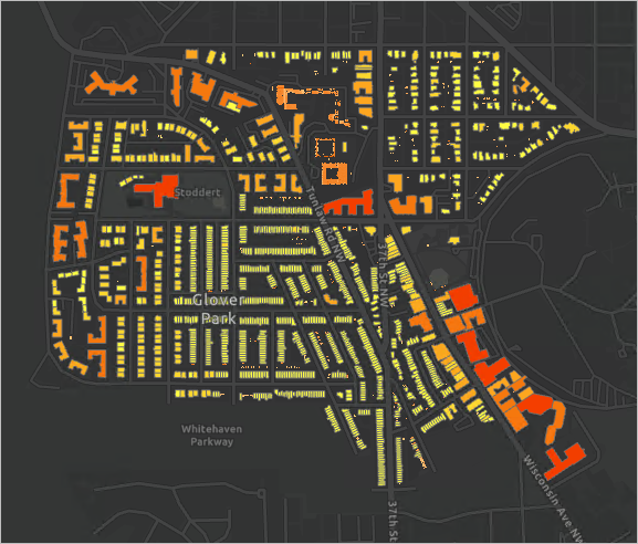
- Explore the final map.
At a glance, the larger buildings tend to have higher electric power production potential than single-unit dwellings. This pattern makes sense, since larger buildings have larger roof surfaces. Note that larger buildings also have higher electric power needs.
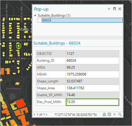
- Click one of the single-unit houses (small buildings).
An informational pop-up appears, showing the attribute values for that building. In the following example image, the electric power production potential is 13.35 MWh per year.
- Click a few more single-unit houses to view their electric power production potential.
In 2022, the average household in the United States consumed 12,194 kWh per year, that is, 12.194 MWh per year. Could many households in the Glover Park neighborhood cover a significant portion of their electric power needs with solar panels?
You can also check the total amount of power that could be produced by the neighborhood.
- If necessary, close any pop-ups.
- In the Contents pane, right-click Suitable_Buildings and choose Attribute Table.
- In the attribute table, right-click the Elec_Prod_MWh column name and choose Visualize Statistics.
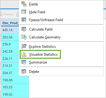
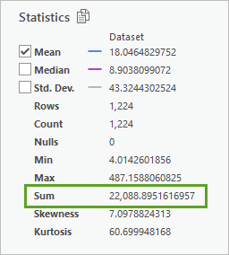
A chart appears, showing the distribution of the field values as a bar chart, as well as a Chart Properties pane. The pane contains statistics, including the sum of electric power production potential for all buildings.
- In the Chart Properties pane, under Statistics, identify the Sum row.
Note:
Your statistics may differ slightly from the example image.
The entire neighborhood has the potential to produce almost 29,000 MWh per year.
- Close the Chart Properties pane, the chart, and the attribute table.
- Press Ctrl+S to save the project.
In this tutorial, you determined the solar power potential of the Glover Park neighborhood in Washington, D.C. To do so, you used a DSM to create a solar radiation raster layer, as well as slope and aspect raster layers. Then, you identified suitable rooftops for solar panels and calculated how much power these rooftops could generate.
Your results represent a yearly average estimate. However, solar-based electric power production varies according to the season, as day length and hours of sunlight change. You could also perform this tutorial's workflow for specific days of the year, such as the winter and summer solstices and the fall and spring equinoxes, to determine the highest, lowest, and medium solar power production values.
Note:
If you want a quicker estimate of the solar radiation per building, you can use the Feature Solar Radiation tool, which computes solar radiation directly for every polygon in a feature layer. However, this shorter workflow won't allow you to differentiate between the suitable and nonsuitable areas within each rooftop.
You can replicate this workflow for any community, as long as you have a building footprints layer and a DSM. Many communities provide open GIS data. The data for this tutorial was acquired from the Open Data DC website. The building footprints layer was downloaded from the site and clipped to the area of interest. A lidar point cloud dataset downloaded from the site was used to derive the DSM. You can learn how to derive a DSM from a lidar point cloud in the Extract 3D buildings from lidar data tutorial.
You can find more tutorials such as this in the Introduction to Imagery & Remote Sensing tutorial collection.

