Download and explore data
Before you can run the deep learning model, you need to check your computer system, install the latest drivers for your graphics card, and install the deep learning libraries that you will use for training and inferencing. Next, you will download three .zip files that contain data that you will use throughout the lesson for training and classification of point cloud data. Once you download and extract the data, you will explore and symbolize LAS dataset files in ArcGIS Pro.
Download the data
All the data required to complete the lesson is in three .zip files that you will now download.
- Before you download the data, ensure that you have the Deep Learning libraries installed and verify that your computer is ready.
Note:
Using the deep learning tools in ArcGIS Pro requires that you have the correct deep learning libraries installed on your computer. If you do not have these files installed, ensure that ArcGIS Pro is closed, and follow the steps delineated in the Get ready for deep learning in ArcGIS Pro instructions. In these instructions, you will also learn how to check whether your computer hardware and software are able to run deep learning workflows and other useful tips. Once done, you can continue with this tutorial.
- On your computer, open the File Explorer.
- In your C:\ drive, create a folder named LearnArcGIS. Within the LearnArcGIS folder, create another folder named DL.
The C:\LearnArcGIS\DL folder is where you will store all the data and outputs for the lesson.
- Download the following .zip files:
- smalldata.zip—Contains a small training dataset and the training boundary, a small validation dataset and the validation boundary, and a DEM raster.
- testdata.zip—Contains a test dataset, the processing boundary, and a DEM raster.
- results.zip—Contains the training results from the large dataset that you can use instead of training the model for the large dataset.
- When the files are downloaded, extract each .zip file to the LearnArcGIS/DL folder.
Note:
To extract a .zip file, right-click it, choose Extract All, and browse to your LearnArcGIS\DL folder.
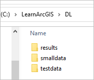
The folders contain various information that you will use for preparing and training data. Some of the main files in the folder are LAS files. A LAS file is an industry-standard binary format for storing airborne lidar data. The LAS dataset allows you to examine LAS files, in their native format, quickly and easily, providing detailed statistics and area coverage of the lidar data contained in the LAS files. The results folder contains a trained model using the large dataset that was performed on a computer with 24 GB GPU. In the final section of this lesson, you will use this trained model later in the lesson to classify a LAS dataset.
Next, you will review and familiarize yourself with the downloaded data in ArcGIS Pro.
View the training data and validation data
You will create an ArcGIS Pro project and view the small training data and validation data.
- If necessary, start ArcGIS Pro.
- Sign in to your ArcGIS organizational account or into ArcGIS Enterprise.
Note:
If you don't have access to ArcGIS Pro or an ArcGIS organizational account, see options for software access.
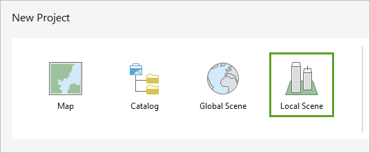
- Under New Project, click Local Scene.
- On the Create a New Project dialog box, for Name, type Powerline Classification with DL. For Location, click Browse, browse to C:\LearnArcGIS, click the DL folder, and click OK. Uncheck Create a new folder for this project.
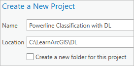
- Click OK.
- In the Catalog pane, expand Folders and expand DL.
Note:
If the Catalog pane is not visible, on the ribbon, click View, and in the Windows group, click Catalog Pane.
You can see the data folders that you downloaded and extracted to this location.
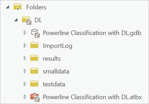
First, you will explore the files in the smalldata folder and update the statistics on the dataset to ensure that the proper class codes display.
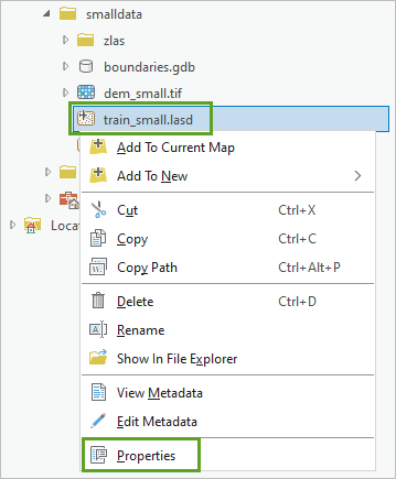
- In the Catalog pane, expand the smalldata folder. Right-click train_small.lasd and choose Properties.
- In the LAS Dataset Properties window, click the Statistics tab.
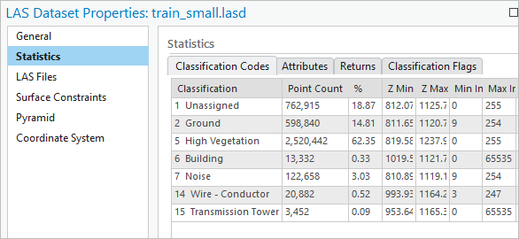
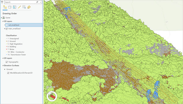
The dataset contains several class codes:
- 1- Unassigned represents unclassified points, mainly low vegetation or objects above the ground, but lower than high vegetation and buildings.
- 2- Ground represents the ground.
- 5- High Vegetation represents high vegetation, such as trees.
- 6- Building represents buildings and other structures.
- 7- Noise represents low points.
- 14- Wire-Conductor represents actual power wires.
- 15- Transmission Tower represents the power line towers.
You are interested in the class code 14 for Wire - Conductor. Your goal is to train a model to detect lidar points that are the power lines so you can better assess wildfire risks for power lines near trees.
At the bottom of the window, there is a message that states that one file has out-of-date or no statistics. You will fix this issue now so that you can display the correct class codes in the scene.
- Click Update.
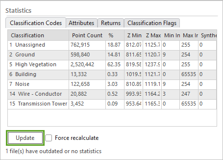
A message appears confirming that the statistics are up to date.
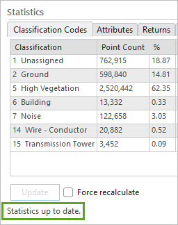
Now that the statistics are up to date, you can style the layer according to class codes.
- Click OK.
- In the Catalog pane, right-click train_small.lasd and choose Add To Current Map.
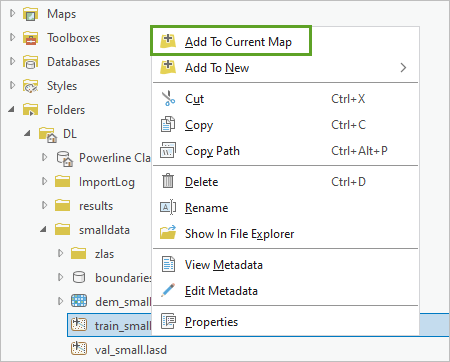
The LAS dataset layer appears in the scene.
Now that you have updated the statistics for the small dataset LAS file, you will do the same for the LAS dataset that will be used to validate the model, val_small.lasd.
- In the Catalog pane, open the properties for val_small.lasd, update the statistics, and click OK. Add val_small.lasd to the current map.
- In the scene, press V or C while dragging your pointer to tilt it and pan the scene to explore the datasets in 3D.
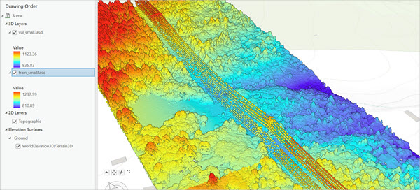
You will use train_small.lasd to train the model and val_small.lasd for validating the trained model to prevent overfitting during the training process.
Next, you will update the symbology for each of the LAS dataset layers to show different colors by the class codes. You'll start with the train_small.lasd layer.
- In the Contents pane, click the train_small.lasd layer to select it. On the ribbon, click the LAS Dataset Layer tab.

- On the LAS Dataset Layer tab, in the Drawing section, for Symbology, click the drop-down menu and choose Class.
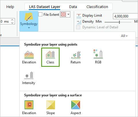
The Symbology pane appears and the train_small.lasd layer is symbolized by its class codes.
Note:
If you have white spaces in your LAS dataset layer, this could be a caching issue. You can go to the properties of the LAS dataset, choose Cache, and click Clear Cache to fix this, or it will be fixed automatically when you close and open ArcGIS Pro.
- In the Contents pane, click val_small.lasd. On the Las Dataset Layer tab, click the drop-down menu for Symbology and choose Class.
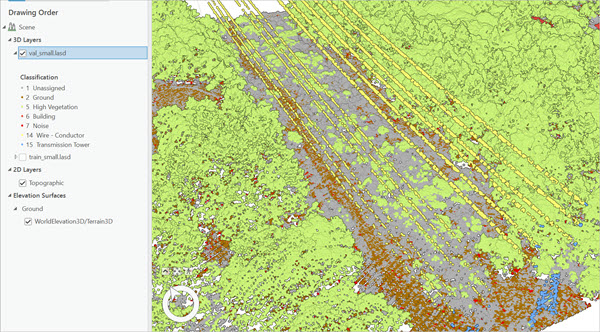
The val_small.lasd layer is now symbolized by its class codes.
Note:
LAS datasets can be large and take more time to display than other layers. To speed up the display, you can build pyramids using the Build LAS Dataset Pyramid tool. This tool creates or updates a LAS dataset display cache, which optimizes its rendering performance.
- Above the ribbon, on the Quick Access toolbar, click Save to save the project.
Next, you will train a model using these two datasets that you explored.
Train a model using a small dataset
In this section, you will use the small datasets to walk through the process of training a classification model. Because this dataset does not contain as many points needed for training a more accurate classification model, it is likely to produce a less accurate classification model. This section shows you the process of training a model and then you will use a trained model from a larger sampling of points later in the lesson to classify a LAS dataset and visualize the power lines.
Prepare the training dataset
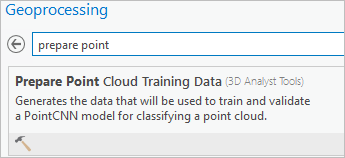
LAS datasets cannot be used directly to train the model. The LAS datasets must be converted into smaller training blocks. You will use the Prepare Point Cloud Training Data geoprocessing tool in ArcGIS Pro to export the LAS files to blocks.
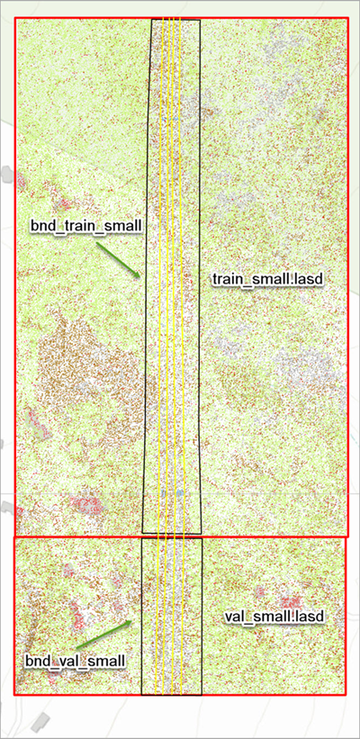
Your goal is to train the model to identify and classify the points that are power lines. Not every point in the LAS data cloud is necessary to review. Only the points within the surrounding area of power lines need to be reviewed. You will use prepared boundary data, bnd_train_small and bnd_val_small, to specify which points should be converted into training blocks. Below is the graph showing the training and validation boundaries surrounding power lines.
- On the ribbon, click the Analysis tab and click Tools.
The Geoprocessing pane appears.
- In the Geoprocessing pane, search for and open the Prepare Point Cloud Training Data tool.
Note:
This tool requires the ArcGIS 3D Analyst extension. - In the Prepare Point Cloud Training Data tool, set the following parameters:
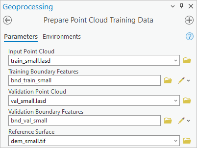
- For Input Point Cloud, choose train_small.lasd.
- For Training Boundary Features, click Browse, browse to C:\LearnArcGIS\DL\smalldata\boundaries.gdb, choose bnd_train_small, and click OK.
- For Validation Point Cloud, choose val_small.lasd.
- For Validation Boundary Features, click Browse, browse to C:\LearnArcGIS\DL\smalldata\boundaries.gdb, choose bnd_val_small, and click OK.
- For Reference Surface, click Browse and browse to C:\LearnArcGIS\DL\smalldata. Click dem_small.tif and click OK.
The DEM raster will be used to calculate points' relative height from the ground. You have entered all the training data, validation data, and processing boundaries.
Next, you will specify which class codes to exclude.
- For Excluded Class Codes, type 2. Click the Add another button and type 7.

Ground (class 2) and noise (class 7) points are excluded from the training data. Ground points typically account for a large portion of the total points so excluding ground points will make the training process more quickly.
- Leave Filter Blocks by Class Code blank.
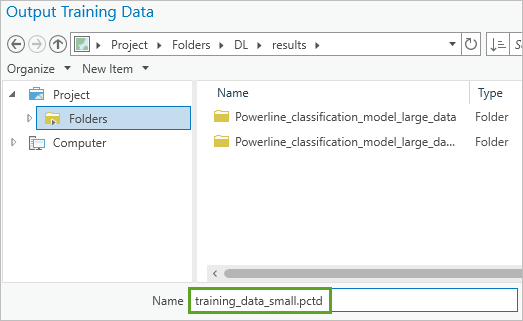
- For Output Training Data, click Browse and browse to C:\LearnArcGIS\DL\results. For Name, type training_data_small.pctd.
Note:
The output file extension .pctd stands for point cloud training data.
- Click Save.
- In the Prepare Point Cloud Training Data tool, continue entering the following parameters:
- For Block Size, type 82. For Unknown, click the drop-down menu and choose US Survey Feet.
- For Block Point Limit, keep the default of 8192.

Block Size and Block Point Limit control how many points are in one block. To determine this value, it is important to consider the average point spacing, the objects of interest, available dedicated GPU memories, and the batch size when setting these two parameters. A general rule is that the block size should be large enough to capture the objects of interest with the least amount of subsampling.
You will start with the Block Size of 82 feet (about 25 meters) and the Block Point Limit of 8192. 82 feet is a proper block size to capture the power line’s geometry. You will examine the output to see if 8,192 is an appropriate block point limit. If most blocks have more than 8,192 points, you will need to increase the block point limit to reduce subsampling.
Note:
For the large data, it is recommended that you use the LAS Point Statistics As Raster tool to generate the histogram to determine the proper block size and block point limit before running the Prepare Point Cloud Training Data tool. To use the tool, choose Point Count as the method and Cell Size as the sampling type and test with different values for Block Size.
- Click Run.
A confirmation message appears at the bottom of the tool pane when the tool completes.
- Click View Details.
Under Messages, you can see two histograms of the block point count, one for the training data and one for the validation data.
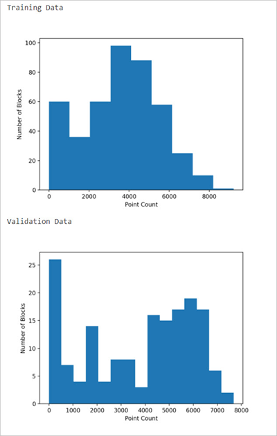
Both histograms show that almost all the blocks have a point count of less than 8,000, which confirms that a Block Size of 82 feet and the default Block Point Limit of 8,192 are proper for these datasets.
- In Windows, open the File Explore and browse to C:\LearnArcGIS\DL\results. The results folder now contains a training_data_small.pctd folder.
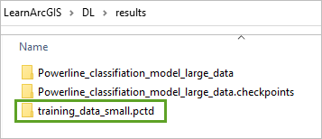
- Double-click training_data_small.pctd to open the folder.

The output file contains two subfolders, train and val, which contain the exported training and validation data, respectively.
- Open each folder to review their contents.
In each folder, you will see a Statistics.json file, a ListTable.h5, a BlockPointCountHistogram.png file, and a 0 folder containing Data_x.h5 files.

The ListTable.h5 and Data_x.h5 files include the information of points (xyz and attributes such as return number, intensity, and so on), which are organized into blocks.
Now that you have prepared the training data, you can use the blocks to train a classification model with deep learning.
Train a classification model
Next, you will use the Train Point Cloud Classification Model geoprocessing tool to train a model for power line classification using the small training dataset. The results may vary based on different runs of the tool and different computer configurations.
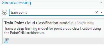
- In ArcGIS Pro, in the Geoprocessing pane, click the back arrow. Search for and open the Train Point Cloud Classification Model tool.
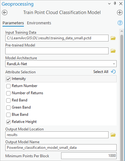
- In the Train Point Cloud Classification Model tool, set the following parameters:
- For Input Training Data, click Browse. Browse to C:\LearnArcGIS\DL\results, and double-click training_data_small.pctd.
- For Pre-trained Model, leave it blank.
- For Model Architecture keep the default of RandLA-Net.
Note:
You will use RandLA-Net architecture to train the classification model. RandLA-Net uses random sampling to reduce memory usage and computational cost and use local feature aggregation to preserve useful features from a wide neighborhood.
- For Attribute Selection, click the check box for Intensity and Relative Height.
Note:
The intensity of power lines is lower when compared with other features, so it is an effective attribute for distinguishing power lines. The relative height of power lines is usually within a certain range, so it is also used to separate powerlines from other features.
- For Output Model Location, browse to the results folder. Click it and click OK.
- For Output Model Name, type Powerline_classification_model_small_data.
- For Minimum Points Per Block, type 1000.
By setting the Minimum Points Per Block to 1000 during the training, blocks whose points are less than 1,000 will be skipped. Blocks with a small number of points are likely to be located at the boundaries where there are no power line points. Skipping these blocks in the training will make the training faster and make the model's learning more efficient. This parameter is only applied on the training data blocks, not the validation data blocks.
- Expand Manage Classes.
- Under Class Remapping, for Current Class, choose 14. For Remapped Class, choose 14.
Class 14 represents the wire conductors that you want to classify and locate in the point cloud.
- In the next row, for Current Class, choose OTHER and from Remapped Class, choose 1.
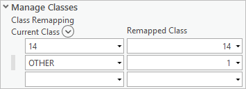
By specifying the Class Remapping, classification code 14 will remain unchanged, meaning points in the LAS dataset that already classify as power lines will remain power lines. All other class codes (1, 5, and 15) will be remapped to the class code of 1. The resulting training data will only have two classes, 1 and 14, thus making the power lines easier to distinguish in the scene.
- For Class Description, accept the populated class codes and descriptions.

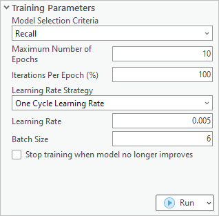
- Expand Training Parameters. For Model Selection Criteria, accept the default of Recall.

Model Selection Criteria specifies the statistical basis that will be used to determine the final model. The default of Recall will select the model that achieves the best macro average of the recall for all class codes. Each class code's recall value is determined by the ratio of correctly classified points (true positives) over all the points that should have been classified with this value (expected positives). For each class, its recall value is the ratio of correctly predicted points of this class to all the reference points of this class in the validation data. For example, the recall value of class code 14 is the ratio of correctly predicted power line points to all the reference power line points in the validation data.
- For Maximum Number of Epochs, type 10.
An epoch is the complete cycle of the entire training data learned by the neural network (in other words, the entire training data is passed forward and backward through the neural network one time). You will train the model for 10 epochs to save time.
- For Iteration Per Epoch (%), accept the default of 100.
Leaving the Iteration Per Epoch (%) parameter at 100 ensures that all the training data will be passed per epoch.
Note:
You can also choose to pass a percentage of the training data at each epoch. Set this parameter to something other than 100 if you want to reduce the completion time for each epoch by randomly selecting fewer batches. However, this can lead to more epochs before the model converges. This parameter is useful is you want to quickly see the model metrics at the tool’s messages window.
- For Learning Rate Strategy, keep the default of One Cycle Learning Rate.
- For Learning Rate, type .005.
Note:
You can also leave Learning Rate blank and let the tool to find an optimal learning rate for you.
- For Batch Size, type 6.
Batch Size specifies how many blocks are processed at a time. The training data is split into batches. For example, if the Batch Size value is set to 20, 1,000 blocks are split into 50 batches, and each of the 50 batches are processed in one epoch. By splitting the blocks into batches, the process will consume less GPU memory.
Note:
Batch size of 20 is recommended on 8 GB graphic card. If you received CUDA out of memory error, you should use a smaller batch size.
- Uncheck Stop training when model no longer improves.
Unchecking this option will allow the training to run for 10 epochs. If checked, the training will stop when the model is no longer improving after several epochs, regardless of the maximum number of epochs specified.
- Click Run.
Note:
Depending on your system, the time it takes to run this tool may vary. On the NVIDIA Quadro RTX 4000 GPU with 8 GB of dedicated memory, this tool will take about 20 minutes to run. As the tool runs, you can monitor its progress.
- At the bottom of the Geoprocessing pane, click View Details.

The Train Point Cloud Classification Model (3D Analyst Tools) window appears, displaying the Parameters tab, which shows the parameters that were used for running the tool.
- Click the Messages tab.
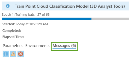
Note:
The geoprocessing messages populate as the tool runs. When the tool is completed, the geoprocessing message shows the results for each epoch.
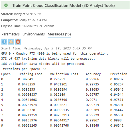
Note:
The information in your messages may be different from the example shown, depending on your GPU and system setup.
The tool reports the following information:
- GPU used in the training.
- Count of the training data blocks used in the training (only training data block containingmore than 1,000 points are used in the training).
- Count of the validation data blocks used in the validation—all the validation data blocks are used in the validation.
- Iteration per epoch—the count of the training data blocks divided by the batch size.
The tool reports Training Loss, Validation Loss, Accuracy, Precision, Recall, F1-Score, and Time spent for each epoch.
As each epoch progresses, you can see the Training Loss and Validation Loss values decrease, which indicates that the model is learning.
After 10 epochs, the highest Recall value is over .98.

This model is not an accurate model, which is expected because the model was trained with a small dataset. These results highlight the need to have more sample points in separate datasets so that you can achieve better results.
Examine the training outputs
Next, you will look at the results of training the classification model.
- In the File Explorer, browse to C:\LearnArcGIS\DL\results.
In this folder, there are two subfolders. One is the model folder, and another is the checkpoints folder.
- Expand the Powerline_classification_model_small_data folder and expand the Model Characteristics folder.
The Powerline_classification_model_small_data folder includes the saved model at the epoch of 9. There are several files inside the model folder. Among them, the .pth file is the model file and the .emd file is Esri Model Definition file (a configuration file in .JSON format). The model_metrics.htm includes a learning loss graph. The .dlpk file is the deep learning model package. It is a compressed file and can be shared at ArcGIS Online.
The Model Characteristics folder contains a loss graph and ground truth and predictions results graph.
- Go back to the results folder. Open the Powerline_classification_model_small_data.checkpoints folder and view its contents.
The Powerline_classification_model_small_data.checkpoints folder includes the models folder, which contains a model for each of the epoch checkpoints and two .csv files. When the training tool was running, one checkpoint was created after each epoch. Each checkpoint contains a .pth file and an .emd file.
- In the Powerline_classification_model_small_data.checkpoints folder, open the Powerline_classification_model_small_data_Epoch_Statistics Microsoft Excel file to see the statistics.
The CSV file opens in Excel.
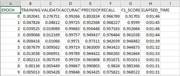
It is the same table that you saw in the tool's message.
The Powerline_classification_model_small_data_Statistics file includes the precision, recall, and f1-score values for each class after each epoch. In certain cases, the model with the best overall metrics may not be the model that performed the best in classifying a specific class code. If you are only interested in classifying certain class codes, you may consider using the checkpoint model associated with the best metrics for that class code. Viewing the statistics in Excel allows you to sort the columns and easily locate the epoch with the highest recall value. You have trained a model using a smaller sampling of points. Next, you will use a model that was trained using a larger sampling of points to classify a LAS dataset.
Classify a LAS dataset using the trained model
You will classify the LAS dataset containing more than 3 million points using a trained model. Classifying the LAS dataset using a trained model allows you to locate power lines in the study area for risk assessment analysis. When the model was trained, two classification codes were designated, Unassigned and Wire Conductor. By classifying points in the point cloud to wire conductor and the rest as unassigned, it will make the dataset more valuable, as it will clearly identify power lines.
Explore model results and choose the best epoch
You will explore the results of a provided model training that used the large dataset. You will look for the best recall value for wire conductors.
- Open the File Explorer and browse to C:\LearnArcGIS\DL\results.
The folders contain results of training a large data using a computer with 24 GB of dedicated GPU memory.
- Open the Powerline_classification_model_large_data.checkpoints folder and double-click Powerline_classification_model_large_data_Statistics to view the statistics in Excel.
The file opens in Excel.
- In Excel, double-click the column dividers to expand them so that you can see all the text.
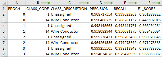
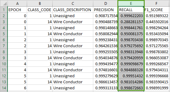
You will sort the Recall column and find the largest value for Wire Conductor and use that epoch for classifying the LAS dataset. The largest Recall value for the Wire Conductor indicates the epoch that you should use in the classification.
- Click the Recall column header to highlight the entire column.
- On the ribbon, in the Editing section, click Sort & Filter and choose Sort Largest to Smallest.
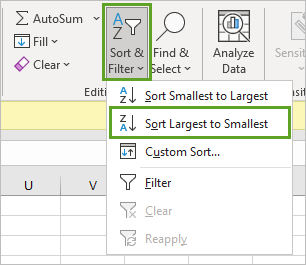
- In the Sort window that appears, click Sort.
The rows in the spreadsheet are sorted so it is easy to see the highest value for Wire Conductor.
- Locate the first row with a CLASS_CODE of 14 and a CLASS_Description of Wire Conductor (row 23).
This is the highest recall value of 0.993655113, for Wire Conductor, which occurred in epoch 18.
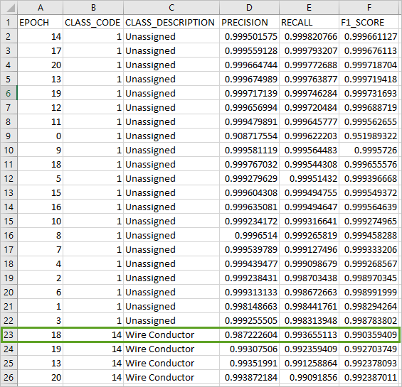
You will use epoch, or checkpoint 18, when you classify the LAS dataset, as it has the highest recall value for the power line class code and will provide the best results.
Classify power lines using the trained model
Next, you will use a trained model to classify the power lines from a test dataset. You will apply processing boundaries to only classify points within the boundaries.
- Restore ArcGIS Pro.
- In the Catalog pane, expand Folders, expand DL, and expand testdata. Open the properties for test.lasd and update the statistics. Click OK.
- Right-click test.lasd, choose Add To New, and choose Local Scene.
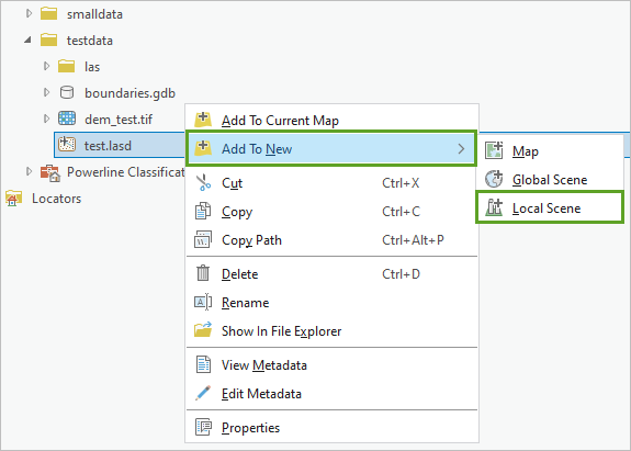
The test.lasd LAS dataset appears in a local scene.
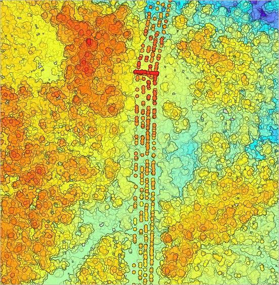
- If necessary, in the Contents pane, click test.lasd to select it. On the ribbon, click the LAS Dataset Layer tab, click the drop-down arrow for Symbology and choose Class.
The test.lasd LAS dataset is now rendered using class codes.
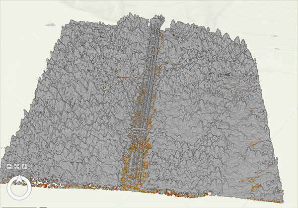
Ground points (class 2) and low noise points (class 7) are already classified. The left points are unassigned (class 1).
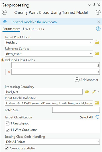
- In the Geoprocessing pane, search for and open the Classify Point Cloud Using Trained Model tool.
- For Target Point Cloud, click the drop-down menu and choose test.lasd.
- For Reference Surface, click the Browse button and browse to C:\LearnArcGIS\DL\testdata. Click dem_test.tif and click OK.
- For Excluded Class Codes, add 2 and 7.
- For Processing Boundary, browse to C:\LearnArcGIS\DL\testdata\boundaries.gdb and double-click bnd_test.
By selecting a Processing Boundary, the tool will use the trained model you provide to classify only the points within the boundary.
Note:
Because the power line classification model was trained using boundaries, a reference surface, and excluding certain class codes, the same parameters should also be set for the Classify Point Cloud Using Trained Model tool.
- For Input Model Definition, click Browse. Browse to the C:\LearnArcGIS\DL\results\Powerline_classification_model_large_data.checkpoints\models\checkpoint_2023-03-28_18-21-34_epoch_18 folder and open it. Click checkpoint_2023-03-28_18-21-34_epoch_18.emd and click OK.
Note:
For Input Model Definition, you can choose an .emd file, a .dlpk file, or the URL to the model shared at ArcGIS Online or ArcGIS Living Atlas of the World.
The Target Classification parameter appears after selecting a model definition file.

Leave the Batch Size blank and let the tool to calculate an optimal batch size for you based on the available GPU memory.
Since class code 2 and 7 are excluded from the classification. The model only classifies the left points (class 1). When the model runs, the points are predicted as power lines and will have their class codes assigned as 14; otherwise, their class codes are kept as 1.
Note:
Ignore the warning appearing at the Excluded Class Codes parameter.
- Click Run.
The tool runs. Next, you will update the symbology to show the results of the classification model.
- In the Symbology pane, next to Value, click More and click Add all values.
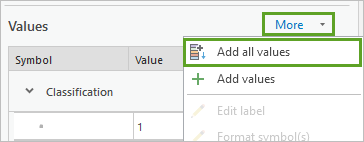
The symbology updates and the points in the point cloud that are wire conductors display in yellow.
- Use the navigation tools and shortcuts to examine the classification results in the local scene.
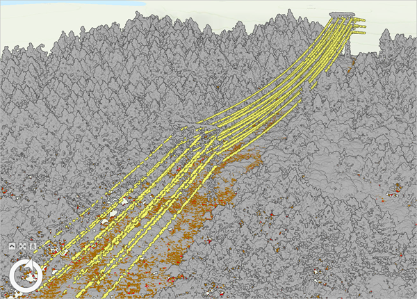
The classification results are accurate using the trained model. Almost all the power line points are correctly classified. Notice that the power poles are still Unassigned.
In this tutorial, you learned the workflow of point cloud classification using deep learning technology. You gained experience with deep learning concepts, the importance of validation data in the training process, and how to evaluate the quality of the trained models. Going further, you can use the Extract Power Lines From Point Cloud tool to generate 3D lines to model the power lines. You could also use the Generate Clearance Surface tool to determine the clearance zone around the power lines. The points within the clearance zone, mostly trees, are too close to the power lines, which could cause a power outage or spark a fire. These tools can go further to provide important information for insurance risk assessments.
You can find more tutorials in the tutorial gallery.


