Prepare for deep learning
Training a model to automatically classify satellite imagery requires that you have the proper deep learning libraries on your computer. First, you'll need to verify that your system has the correct settings and libraries.Then, you'll download Landsat 8 imagery and create training labels that indicate where mangroves are present in the image. Finally, you'll export these labels to train a pixel classification deep learning model.
Set up and download the tutorial data
Verify that your machine is correctly set up to do deep learning, then you'll download the data needed for this tutorial. It includes Landsat 8 imagery and mangrove forest locations from the United Nations' Global Mangrove Watch.
- Before you can use the deep learning tools, ensure that your machine is ready.
Note:
Using the deep learning tools in ArcGIS Pro requires that you have the correct deep learning libraries installed on your computer. If you do not have these files installed, ensure that ArcGIS Pro is closed, and follow the steps delineated in the Get ready for deep learning in ArcGIS Pro instructions. In these instructions, you will also learn how to check whether your computer hardware and software are able to run deep learning workflows and other useful tips. Once done, you can continue with this tutorial.
- Download the Classify_Mangroves_Tutorial_Data.zip file for this tutorial to a suitable location on your computer and extract its contents.
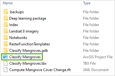
- In File Explorer, open Classify_Mangroves_Tutorial_Data. Open Classify Mangroves.
- Double-click the Classify Mangroves ArcGIS Pro project file.
ArcGIS Pro opens, showing a map of the Mumbai, India, region.
- On the ribbon, click the View tab. In the Windows group, click the Catalog Pane button.
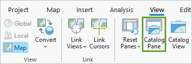
The Catalog pane appears.
- In the Catalog pane, expand Folders. Expand Classify Mangroves.
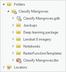
This is the project's file directory.
- Expand the Landsat 8 imagery folder and expand the Landsat imagery 2016 folder.
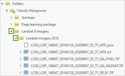
Landsat imagery is provided as a series of files.
Note:
Additional Landsat 8 imagery can be downloaded from the United States Geological Survey's EarthExplorer app. Additional mangrove locations can be downloaded from the Global Mangrove Watch.
- Expand the LC08_L2SP_148047_20160128_20200907_02_T1_MTL.txt item.
Note:
It is the second item in the folder and denoted with a satellite icon.
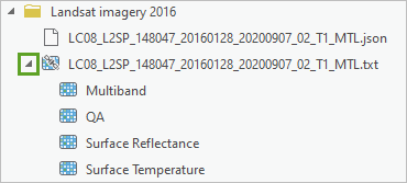
The different Landsat products are visible and can be added to a map. You'll use Surface Reflectance, which is color imagery.
- Right-click Surface Reflectance and choose Add To Current Map.
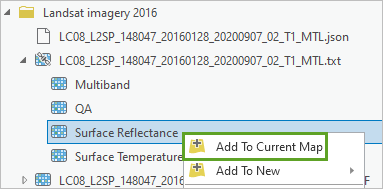
- If the Calculate Statistics window appears, click Yes.
After statistics are calculated, the Landsat imagery is added to the map and to the Contents pane.
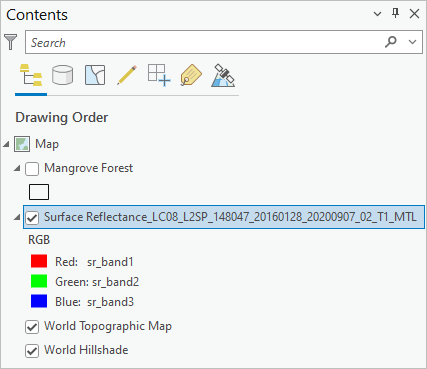
- In the Contents pane, double-click the Surface Reflectance_LC08_L2SP_148047_20160128_20200907_02_T1_MTL layer.
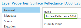
The Layer Properties window appears. You'll rename the layer to shorten it.
- In the General tab, for Name, type Surface Reflectance 2016.
Next, you'll observe the resolution of the Landsat imagery. Resolution is important when you prepare to train the deep learning model.
- In the Layer Properties window, click the Source tab.
- Expand Raster Information.
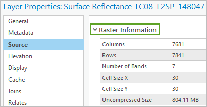
Next to Cell Size X and Cell Size Y, you'll see that this raster's resolution is 30x30. Next, you'll determine the unit of measurement for the cell size.
- Expand Spatial Reference.
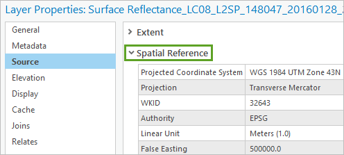
The Linear Unit value is Meters. The resolution of this raster is 30 meters. This means that each pixel in the Landsat imagery measures 30 meters by 30 meters on the ground.
- Click OK.
- On the Quick Access Toolbar, click Save.

You downloaded an ArcGIS Pro project and added Landsat 8 imagery to it. Next, you'll use these datasets to train a model that will be used to classify mangrove forests automatically.
Train a deep learning model
Training a deep learning model requires converting GIS data into a format that can be used to classify imagery. First, using imagery from 2016, you'll mark the locations of mangroves manually. These marked locations are known as labels. Then these labels that you identified will be used to train the model. After the model is created, you'll apply it to 2021 imagery to automatically classify mangrove forests.
Note:
Mangrove locations have been provided to you from the United Nations. You can choose to use the provided dataset or create your own labels by following the steps below. If you want to use the provided mangrove dataset, skip ahead to the Export training data section of this tutorial.
Prepare the training labels
First, you'll create labels. These labels are areas on the imagery that you know contain mangroves. They can be created by manually digitizing, or drawing, polygons on the imagery.
- On the ribbon, click the Map tab. In the Navigate group, click Bookmarks and choose Mangroves.
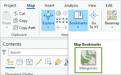
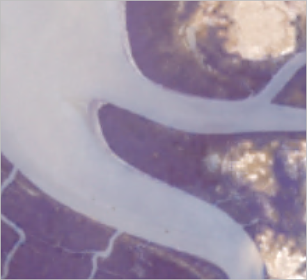
An area with mangroves appears on the map.
- On the ribbon, click the Imagery tab. In the Image Classification group, click Classification Tools and choose Training Samples Manager.
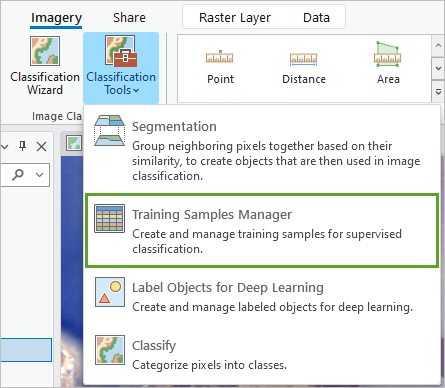
The Image Classification pane appears. This pane allows you to create different classes for the varying features that you want the model to classify in the imagery. You'll add a class that will be used for mangroves. This class will be stored in a custom schema.
- In the Image Classification pane, click Create New Schema.
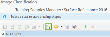
The default schema is removed.
- Click the Add New Class button.
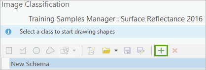
Note:
If you cannot see the Add New Class button, increase the width of the Image Classification pane.
First, you'll give the class a name.
- For Name, type mangrove.

Next, you'll assign this class a value. The computer will read this value when the model is trained. Mangroves will be defined with a value of 1.
- For Value, type 1.

Finally, you'll provide the class with a color. You'll use this color when the areas of mangroves are digitized on the imagery. Black is easily visible on the imagery for this project.
- For Color, choose Black.
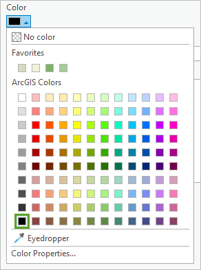
- Click OK.
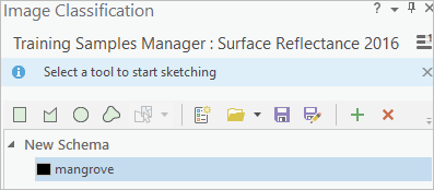
The mangrove class is now available in your new schema. You'll save this change you made to the schema before using it.
- Above New Schema, click Save.

- For Name, type Mangrove classification.

- For Description, type Schema used to label mangroves from Landsat 8 imagery.

- For Output Location, browse to the Classify Mangroves folder and click OK.

- Click Save.
The new schema and mangrove class have been saved.
- Save your project.
The schema is saved and can be used by other users or for other projects.
Create the training labels
Now that you have created a new label class, you'll use it to digitize areas of mangrove forests in the map.
- Under Mangrove classification, click mangrove.
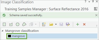
The class becomes active. Next, you'll choose how you want to digitize areas of mangroves on the imagery.
- Click the Polygon tool.
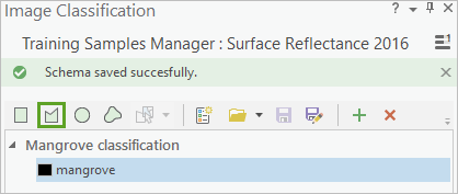
You have selected the mangrove class and an appropriate drawing tool. You'll now begin to mark areas of mangroves on the imagery.
- On the map, click once to begin delineating an area of mangroves. Continue clicking to add vertices and create an enclosed area. Double-click when you're done drawing your first area.
Note:
To cancel your polygon while digitizing, press the Esc key.
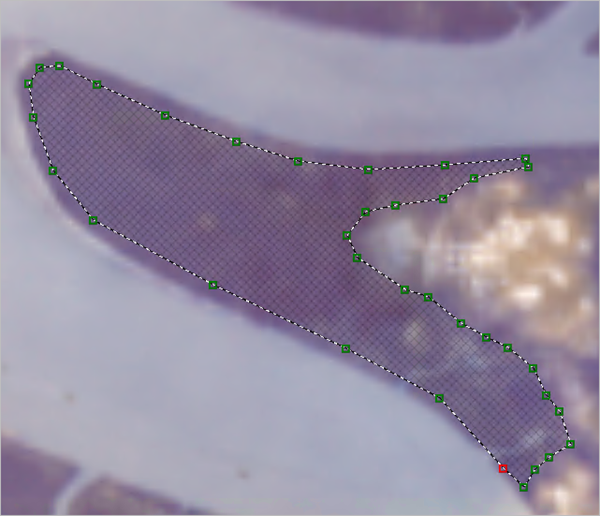
The completed feature has a black outline.
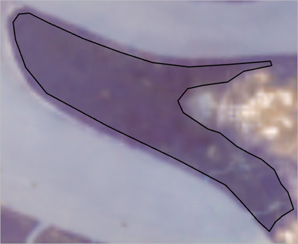
For your final model to have the best results, it is recommended that you digitize as many areas of mangroves as you can. You also want to ensure that the areas you digitize contain only mangrove forests.
Continue delineating areas of mangroves from the imagery. When you're finished digitizing labels, you'll save your results in a geodatabase.
- In the Image Classification pane, above Class, click Save.

You're asked to save your polygons as a feature class. You'll save them to your project's default geodatabase.
- In the Save current training samples window, under Project, expand Databases. Click Classify Mangroves.gdb.
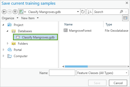
- For Name, type mangrove, and click Save.
Your digitized areas are saved. You'll now remove the training samples from the map.
- Close the Image Classification pane.
The Training Samples Manager window appears asking you to save your edits.
- Click Yes.
Your geodatabase needs to be refreshed for your new feature class to appear.
- In the Catalog pane, expand Databases. Expand Classify Mangroves.gdb.
- Select Classify Mangroves.gdb and press F5.
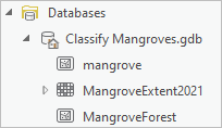
Your geodatabase is refreshed and the mangroves layer now appears as a feature class. However, this data needs to be converted to the proper format for model training.
Export training data
Now that the training data has been created, you'll use the Export Training Data for Deep Learning geoprocessing tool to convert the data into a format that can be used for deep learning. The output of this process is referred to as image chips. The Landsat imagery will be broken into these chips, or small tiles, that will be used to train the model. This first geoprocessing tool will determine how those chips are produced.
- On the ribbon, in Command Search, type Export Training Data For Deep Learning. In the list of search results, choose Export Training Data For Deep Learning.
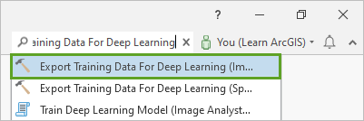
The Geoprocessing pane appears. First, you'll choose the imagery that'll be used for training.
- For Input Raster, choose Surface Reflectance 2016.

Next, you'll create a folder that will hold your training data.
- For Output Folder, browse to the Classify Mangroves folder. Right-click Classify Mangroves and choose Folder.
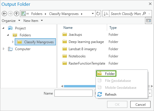
- For the name of the folder, type MangroveTrainingData.
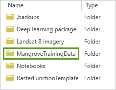
- Select the folder and click OK.
Next, you'll choose the feature class you created earlier that defines the areas of mangroves on the imagery.
- For Input Feature Class Or Classified Raster Or Table, browse to the Classify Mangroves geodatabase and choose the mangrove feature class.
Note:
If you did not create your own mangrove feature class with the Training Samples Manager, choose the MangroveForest feature class.
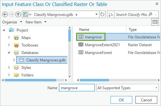
- Click OK.

- For Class Value Field, choose Classvalue.
Note:
If you're using the MangroveForest feature class, choose the pxlval field.

The next set of parameters, Tile Size, will be left with their default values. However, these values can be used to make the chips created by this tool bigger or smaller. The default size is 256x256 pixels. Stride determines how much overlap there is between the chips that are created. By default, each chip overlaps by 128 pixels or 50 percent. Increased overlap will increase the number of chips created.
The last parameter for this tool is Metadata Format. This parameter determines the type of deep learning model you can produce. Since you are doing a pixel classification of mangroves, you'll choose the Classified Tiles format.
- For Metadata Format, choose Classified Tiles.
Finally, you'll set the output cell size of the training data to 30 meters. This resolution is the same as the Landsat 8 imagery.
- Under Export Training Data For Deep Learning, click the Environments tab.

- Under Raster Analysis, for Cell Size, type 30.
- Click Run.
The geoprocessing tool will slice the imagery into chips using the correct format for pixel classification. The slicing is necessary because the full imagery would not fit into most computers' memory all at once. The tool also knows which areas in the imagery are mangroves based on the areas you digitized.
Next, you'll explore the outputs of the tool.
- In the Catalog pane, expand the MangroveTrainingData folder and the images folder.
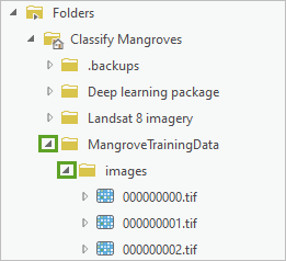
The image files are the chips that were created.
- Right-click the 000000000.tif file and choose Add To Current Map.
- If the Calculate Statistics window appears, click Yes.
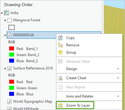
- In the Contents pane, right-click 000000000.tif and choose Zoom To Layer.
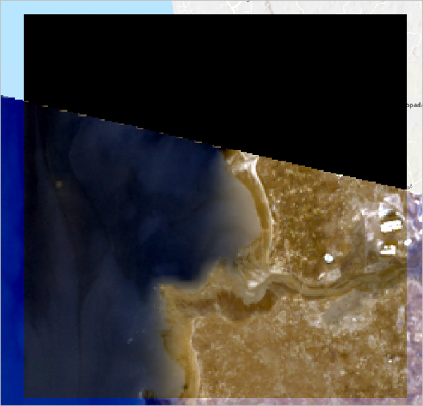
The tile is visible on the map. It is a small piece of the Landsat imagery.
Note:
The image shown is based upon using the MangrovesForest feature class as an input for the Export Training Data for Deep Learning tool. If you chose to digitize your own areas of mangroves, your chips will look different. You may have to add a few chips before you find one with areas of white representing mangrove forests.
Train the model
So far, you've digitized areas of mangroves and exported it to a format that can be used for training. Now, you'll train the model.
Note:
Depending on your computer's hardware, training the model can take up to several hours. It is recommended that your computer be equipped with a dedicated Graphics Processing Unit (GPU). If you do not wish to train the model, a deep learning package has already been provided to you in the Classify Mangroves folder and you may skip to the next section, Deploy the deep learning model.
- On the ribbon, in Command Search, type Train Deep Learning Model. In the list of search results, choose Train Deep Learning Model.
The Geoprocessing pane appears. First, you'll select your training data and then set some deep learning model parameters.
- For Input Training Data, browse to the Classify Mangroves folder and click the MangroveTrainingData folder. Click OK.

Next, you'll choose where to save your deep learning model.
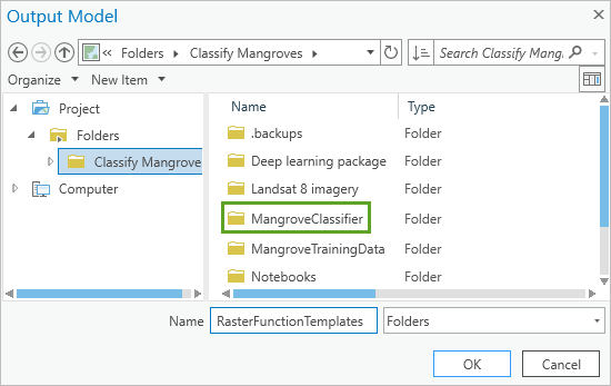
- For Output Model, browse to the Classify Mangroves folder. Create a new folder and name it MangroveClassifier.
- Select the MangroveClassifier folder and click OK.
Now, you'll determine the number of iterations, known as epochs, that the model will run.
- For Max Epochs, confirm that the value is 20.

Based on the format of the training data you exported earlier, you'll set a model type that is specific to pixel classification.
- Expand Model Parameters and confirm that Model Type is U-Net (Pixel classification).

U-Net is a deep learning model that classifies pixels in a raster using semantic segmentation. This model is used for land cover classification.
Next, you'll set the number of training samples to be processed for training one at a time. An increased batch size will process your training data faster.
- For Batch Size, type 16.

Next, you'll change a parameter to ensure that the training runs for all 20 epochs.
- Expand Advanced and uncheck the Stop when model stops improving box.

Finally, if you have a GPU, you'll set this tool to run on your computer's GPU for faster processing. Otherwise, skip the next step.
- Optionally, if your computer has a GPU, click the Environments tab. For Processor Type, choose GPU.

- Click Run.
Note:
If the model fails to run, you may have to adjust the Batch Size parameter. The ability to process larger batch sizes is based upon your computer's GPU. If you have a powerful GPU, you can process up to 64 training samples at a time. If you have a less powerful GPU, you may have to set this parameter to 8, 4, or 2 and rerun the tool.
While the tool is running you can see the training progress.
- Click View Details.

The Details window appears.
- Click the Messages tab.
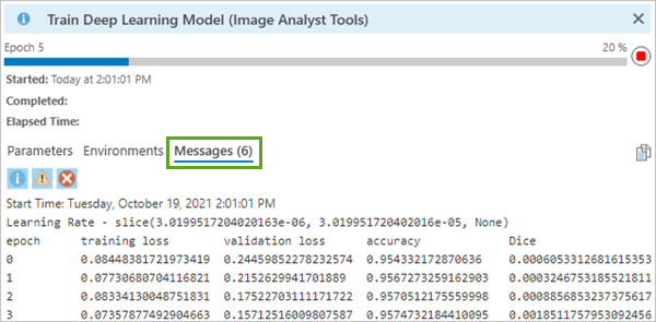
For each of the 20 epochs that run, Messages displays the model's performance. Specifically, you'll begin to see the accuracy of the model increase or move toward 1.
Note:
Since the model trains differently each time this tool is run, your model's messages may vary from the image above.
- Close the Train Deep Learning Model window.

When the geoprocessing tool completes, you'll observe the outputs.
- In File Explorer, browse to your project's folder. Open the MangroveClassifier folder.
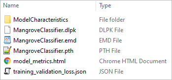
The folder contains a number of outputs that you can used to classify imagery:
- MangroveClassifier.pth is a trained model and is usually saved in a PyTorch format.
- MangroveClassifier.emd is a model definition file that contains model information about the tile size, classes, and model type.
- model_metrics.html contains details about the learning rate used and the final accuracy of the model.
- MangroveClassifier.dlpk is a complete package of all the files stored in model output folder including the trained model, the model definition file, and the model metrics file. This package can be shared to ArcGIS Online and ArcGIS Enterprise as an item for others to access.
You'll explore the model_metrics file to see how your model performed.
- Open the model_metrics file.
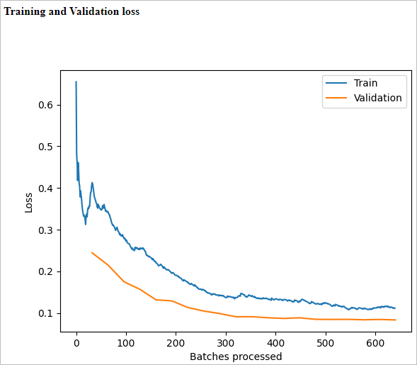
Your default web browser appears. On this page is the information about your model and how well it was able to classify mangroves with your input training data.
The Training and Validation loss section displays a graph of the amount of error that was present as the model trained over time. When the model ran, some of your input data was used to train the model and some was used to validate the model or test the model to determine its accuracy. Ideally, you would see these values decrease as the number of images processed increases over the course of the 20 epochs.
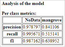
Analysis of the model displays the precision of the classes of data. Your model technically had two classes: one for mangrove and one for NoData. A higher precision value means the model is more confident in its results.
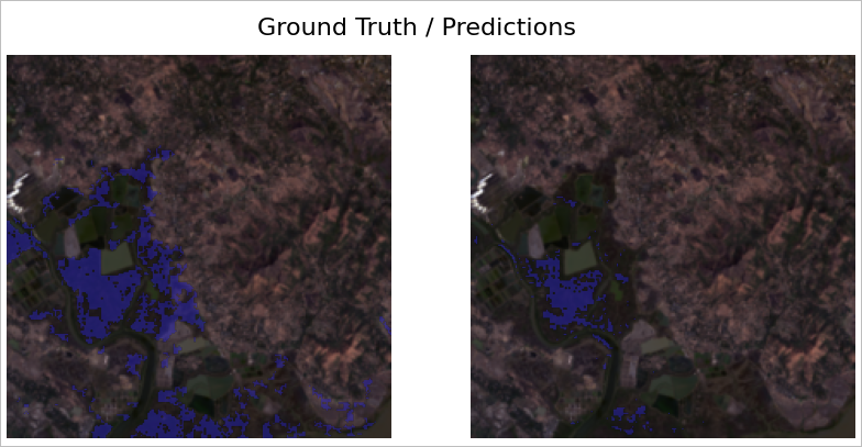
Finally, this page shows a few sample chips comparing your original mangrove training data, Ground Truth, on the left and the model's Predictions on the right. Ideally, the prediction should closely match the original ground truth.
- Close the model_metrics page on your web browser.
- Close File Explorer.
Before deploying your model, you'll clear your GPU's cache to ensure that it has enough memory to classify the 2021 Landsat imagery. If you do not have a GPU on your computer, you may skip this step.
- In ArcGIS Pro, in the Catalog pane, expand Toolboxes. Expand Classify Mangroves.tbx.
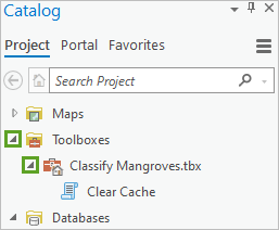
The provided script in this toolbox does not have any inputs.
- Open the Clear Cache script and click Run.
- Save your project.
You created a training model by digitizing areas of mangroves from Landsat 8 imagery taken in 2016. Then, you took your mangroves feature class, converted it to a format suitable for training a deep learning model, and used it to create a deep learning package. Next, you'll use your new model to automatically classify mangroves in Landsat 8 imagery taken in 2021.
Apply the model
Once a deep learning model is created, it can be used repeatedly to quickly classify land cover in an area of interest. You'll take the model that you made and use it to classify mangroves in the same geographic area as your original training data. However, the Landsat imagery will be more recent.
Deploy the deep learning model
Now, you'll take Landsat imagery from 2021 and use your deep learning model to inference, or classify the imagery, and find the extent of mangroves.
Note:
If you did not train a model in the previous module, a deep learning package has been provided for you to use in the Classify Mangroves folder.
Classifying imagery is a GPU-intensive process and can take a while to complete depending your computer's hardware. A classified raster of mangrove locations has been provided in the Classify Mangroves.gdb. If you choose to not classify the imagery, you may skip ahead to Explore results section.
- In the Contents pane, remove the Surface Reflectance 2016 layer.
- In the Catalog pane, expand the Landsat 8 imagery folder. Expand the Landsat imagery 2021 folder.
- Expand the LC08_L2SP_148047_20201224_20210310_02_T1_MTL.txt file.
Note:
It is the second item in the folder and denoted with a satellite icon.
- Add the Surface Reflectance raster to the map. If asked to calculate statistics, click Yes.
- In the Contents pane, rename the Surface Reflectance_LC08_L2SP_148047_20201224_20210310_02_T1_MTL layer to Surface Reflectance 2021.
- Right-click Surface Reflectance 2021 and choose Zoom To Layer.
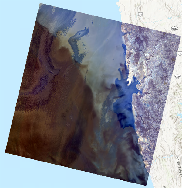
Your 2021 imagery is on the map and ready to be classified. You'll use the Classify Pixels Using Deep Learning geoprocessing tool to apply your deep learning model to this imagery.
- On the ribbon, in Command Search, type Classify Pixels Using Deep Learning. In the list of search results, choose Classify Pixels Using Deep Learning.
- For Input Raster, choose Surface Reflectance 2021.

- For Output Raster Dataset, type MangroveExtent2021.

- For Model Definition, browse to the MangroveClassifier folder. Click the MangroveClassifier deep learning package.

Note:
If you did not train a deep learning model, browse to the Classify Mangroves folder, and open the Deep learning package folder. Click MangroveClassifier.
- Click OK.

There are other model arguments that can be set to improve your model if needed. These parameters carried through from when you trained the model.
- Under Arguments, for batch_size, type 16.

Finally, you'll set the tool's environments.
- Click the Environments tab.
- Under Raster Analysis, for Cell Size, type 30.
- Under Processor Type, set Processor Type to GPU.
- Click Run.
Note:
The ability to set the batch size to 16 depends on your GPU. If the tool fails to run, try changing this parameter to 8, 4, or 2.
When the tool finishes, the results are added to the map.
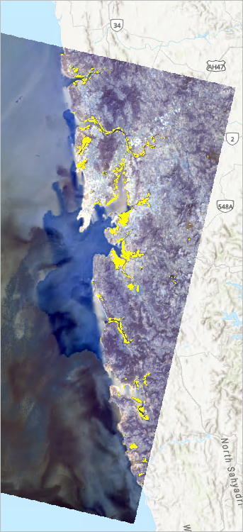
Note:
Depending on your model's accuracy, your results will vary. The color may also vary as well.
Explore the results
Before you begin to compare the mangrove coverage change over time, you'll explore how well your model's results compare to the imagery.
Note:
If you didn't run the Classify Pixels Using Deep Learning tool in the previous section, the results are provided for you. In the Catalog pane, expand Classify Mangroves.gdb. Add the MangroveExtent2021 raster to the map.
- Go to the Mangroves bookmark.
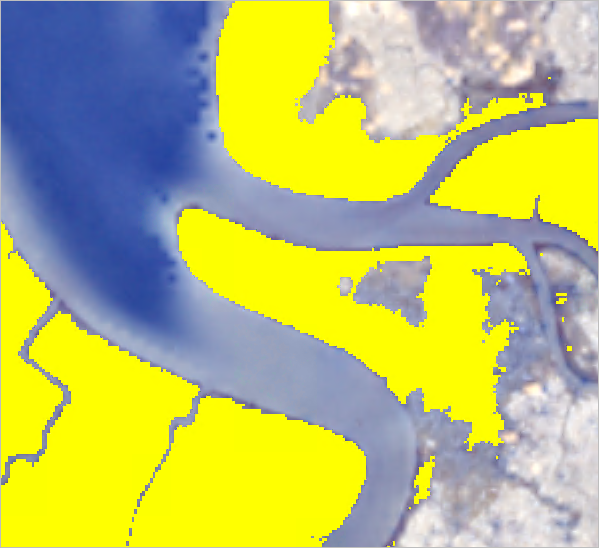
- In the Contents pane, rename MangroveExtent2021 to Mangrove Extent 2021, and keep the layer selected.
- On the ribbon, click the Raster Layer tab. In the Compare group, click Swipe.

The Swipe tool allows you to click and move the map to conceal one layer, revealing the layer under it.
- On the map, drag to reveal the Surface Reflectance 2021 layer under the Mangrove Extent 2021 layer.
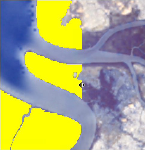
Swiping the map and comparing the two layers helps you visualize your model's results.
Note:
Depending on where you place your pointer on the screen, you can swipe vertically or horizontally.
Before moving on, you'll switch back to the Explore tool, which allows you to move around the map.
- On the ribbon, click the Map tab. In the Navigate group, click the Explore button.
- Save your project.
Now that you have completed the process of training and using a deep learning workflow, you'll compare these results to the mangrove extent from 2016.
Detect changes
To better understand how or where mangrove forests are threatened or growing, you'll perform a raster analysis between the 2016 and 2021 mangrove extents to see where these forests are growing or receding.
Rasterize training labels
To see where mangrove cover is changing, you'll need both of your mangrove layers to be in a raster format. The output layer from the deep learning model is already a raster, but data provided by the Global Mangrove Watch for 2016 mangrove extents is not. You'll convert this polygon layer of mangroves from 2016 into a raster.
- In the Contents pane, turn on the Mangrove Forest layer and turn off the Mangrove Extent 2021 layer.
You can see the outline of mangrove coverage from 2016.
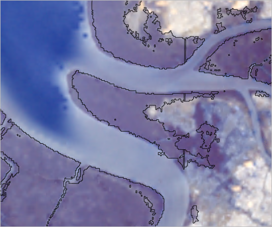
This is the layer that you'll convert to a raster.
- On the ribbon, click the Imagery tab. In the Analysis group, click the Raster Functions button.

The Raster Functions pane appears. Raster functions allow you to create and analyze raster datasets.
- In the search box, type Rasterize Features. Press Enter.

- Under Conversion, click Rasterize Features.
The Rasterize Features raster function appears. First, you'll pick a raster that sets the output raster's extent and resolution.
- For Raster, choose Surface Reflectance 2021.

Next, you'll choose the polygon layer that you want to convert to a raster.
- For Input Features, choose Mangrove Forest.

You'll set the field that classifies each polygon feature as mangroves with a value of 1.
- For Field, choose pxlval.

- Click Create new layer.
- Turn off the Mangrove Forest layer.
A new raster layer of the 2016 mangrove forests is added to the map.
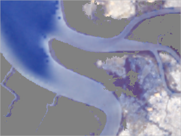
- Rename Rasterize Features_Surface Reflectance 2021 to Mangrove Extent 2016.
Compare mangrove extents
Now that you have two rasters representing the extents of mangroves in 2016 and 2021, you'll use a series of raster functions in a prebuilt template to compare the two extents of mangrove forests to see where they have increased, decreased, or remained the same. Before running the template, you'll explore how it operates.
First, you'll import the raster function template.
- In the Raster Functions pane, clear the search.

- Click the Custom tab.

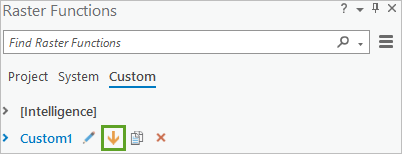
- Point to Custom1 and click Import functions.
- Browse to the Classify Mangroves folder. Select the Compute Mangrove Cover Change raster function template. Click OK.
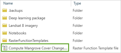
The template is added under Custom1.
- Under Custom1, right-click Compute Mangrove Cover Change. Click Edit.
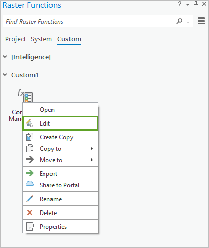
The Function Editor window opens with the Compute Mangrove Cover Change template.
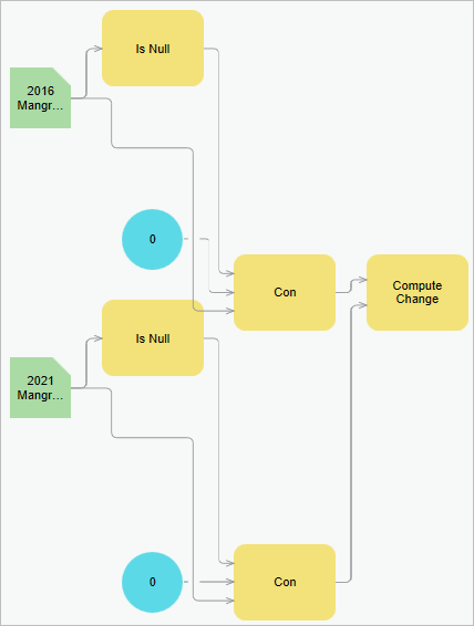
The template starts with the green elements on the left. These represent your two mangrove rasters that'll be compared. Both rasters are linked to an Is Null raster function. This reads the input rasters and determines the areas that have been classified as mangroves and those that are classified as no data. Next, the Con raster function converts the areas of no data to have a value of 0. The mangroves still have a value of 1, which you set when you built your training samples earlier in the tutorial. At this point there are still two rasters, one for 2016 and one for 2021, but now they are binary rasters where the areas of mangroves have an assigned value of 1 and the non-mangrove areas have a value of 0. The final function, Compute Change, subtracts the 2021 mangrove raster from the 2016 raster. Since the areas of mangroves and non-mangroves have been converted to 0s and 1s, the output reveals areas that have seen an increase in mangrove coverage (a value of 1), areas that have seen a decrease in mangrove coverage (a value of -1), and areas that haven't changed (a value of 0).
- Close the Function Editor window.
- In the Raster Functions pane, click the Compute Mangrove Cover Change template.
The raster function appears. You'll configure this tool to run in the same way you would a geoprocessing tool.
- Under Is Null, set 2016 Mangroves to Mangrove Extent 2016.

- Under Is Null, set 2021 Mangroves to Mangrove Extent 2021.

- Click Create new layer.
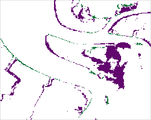
A new layer is added to the map. It depicts areas in purple that saw an increase in mangrove coverage and shows areas in green that lost mangroves. The area in white saw no change. You'll adjust the symbology to make this clearer.
Note:
Your results will vary depending on the results of your deep learning model.
- In the Contents pane, rename Compute Mangrove Cover Change_Mangrove Extent 2016_Mangrove Extent 2021 to Mangrove Cover Change.
- Right-click the Mangrove Cover Change layer and click Symbology.
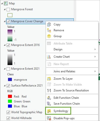
The Symbology pane appears. Next, you'll configure the symbology and remove the white areas with a value of 0.
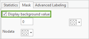
- Click the Mask tab.
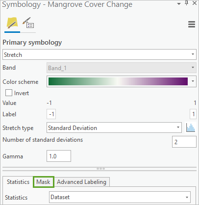
- Check the Display background value box.
The map symbology updates.
- In the Contents pane, turn off the Mangrove Extent 2016 layer.
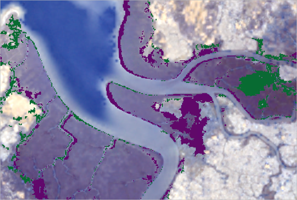
The final results are visible but difficult to see on the imagery. You'll change the transparency of the imagery to make your results clearer.
- In the Contents pane, select the Surface Reflectance 2021 layer.
- On the ribbon, click the Raster Layer tab. In the Effects group, for Transparency type 50 and press Enter.

The final results are now easier to see.
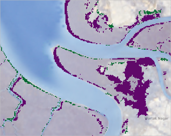
The results from this analysis show where mangrove coverage has increased and decreased between 2016 and 2021. Choosing the right symbology reveals these patterns, making it easier to see these land cover changes over time.
Note:
Exporting samples, training models, and deploying deep learning models can also be done using ArcGIS Notebooks with ArcGIS API for Python and the arcgis.learn module. To see samples of how these geoprocessing tools can be used to process imagery in a notebook environment, go to the Catalog pane and expand the Notebooks folder. You'll see four sample notebooks that use the same processes that you applied in this tutorial.
In this tutorial, you used imagery to create a deep learning model and then applied it. First, you created a training dataset, and this was converted to a pixel classification format. You trained a model to recognize mangroves in Landsat 8 imagery. Then, you applied the model to more recent imagery. Finally, the change in mangrove forests was displayed on the map to make it clear where this tree species is expanding and where it is being lost. These results can be used to help plan mangrove restoration and conservation efforts. Additionally, your deep learning model can be used to classify mangrove habitats all around the world.
Aside from classifying mangroves, Esri provides a number of pretrained models in the ArcGIS Living Atlas to expedite the process of classifying imagery and detecting objects. These models are free to download and you can deploy them directly on compatible imagery inputs. You can also fine tune these pretrained models on your own training data; this usually takes less time than training a model from scratch.
You can find more tutorials in the tutorial gallery.

